SiC Cascodes Show Immunity to Avalanche, Loss of ZVS, and Divergent Oscillations

September 13, 2018, 4:08 am

≫ Next: The Power of Transistor Density: A Look at AMD, Intel, and How Moore’s Law Is Affecting the Market

≪ Previous: BrainChip to Release Biologically Inspired Neurmorphic System-on-a-Chip for AI Acceleration

This article explores how SiC cascodes perform in difficult conditions—including avalanche mode and divergent oscillations—and looks at their performance in circuits that utilize zero voltage switching.

Silicon Carbide (SiC) cascodes have an edge with major characteristics like normalized ON-resistance to chip area (RDSA), device capacitances, and ease of gate drive. However, designers are a cautious lot and understand that headlines are not always the full story. We are naturally wary of changing away from technologies that have proven to be robust over decades, as with IGBTs for example, but what these devices do under real dynamic conditions of voltage stress and external faults is an area of particular concern.

Out-Running the Avalanche

The beauty of a cascode is the use of a low voltage Si-MOSFET which, in conjunction with a normally-ON SiC JFET, gives the device its overall low ON-resistance, fast body diode, and easy gate drive (Figure 1).

Figure 1. SiC cascode

Some might worry that dynamically, the MOSFET could see high drain voltages and enter avalanche mode in normal operation when driven OFF. Could this result in extra losses or even device failure? In cascodes formed with lateral-construction GaN HEMT cells, this is a real possibility as the finite drain-source capacitance CDS of the GaN device forms a ‘pot-down’ with the CDS of the Si-MOSFET and can dynamically leave a high voltage on the MOSFET drain (Figure 2). The SiC JFETs in SiC cascodes are different though, with their vertical ‘trench’ construction, the SiC-JFET CDS value is vanishingly small so that the Si-MOSFET never practically sees the high voltage from the pot-down effect.

Figure 2. Cascode arrangement of Si MOSFET and GaN HEMT cell with voltage dynamically ‘potted-down’ leaving a high voltage on the Si-MOSFET drain

Embracing the Avalanche

There are occasions though when avalanche is desirable, protecting the device from transients produced by inductive loads. GaN cascodes have no avalanche rating and will simply fail with overvoltage whereas the gate-drain diode of the SiC cascode JFET breaks over, passing current through RG, dropping voltage to turn the JFET ON. The Si-MOSFET does now avalanche, but in a controlled way if avalanche diodes are built into each cell. To allay any worries that this intentional avalanche effect is possibly damaging, manufacturers like UnitedSiC prove the point with parts qualified to 1000 hours of operation biased into avalanche at 150°C. As an additional confidence measure, all UnitedSiC parts are subjected to 100% avalanche at final test.

SiC Cascodes Maintain Zero Voltage Switching

Another situation in which the low C_DS of the SiC-cascode scores is in circuits that utilize zero voltage switching (ZVS); a power switch is only allowed to change state when the load voltage has resonantly swung down to zero volts, giving a lossless transition (Figure 3).

Figure 3. Transition as voltage rings down gives zero voltage switching

If the C_DS value of the high voltage switch in a cascode is high, there is a danger that induced current through it can discharge its gate-source capacitance along with the Si-MOSFET drain-source capacitance, turning the high voltage switch prematurely ON before the drain voltage has swung to zero. In this case, ZVS is lost and power is dissipated. The absence of CDS in the SiC-Cascode JFET means that the effect cannot happen.

Divergent Oscillations

A similar effect called divergent oscillation was identified when cascodes were first assembled with discrete devices for the high and low voltage switches. The different technology devices in separate packages and from typically different manufacturers had naturally high stray capacitances and connection inductances which had their own tolerances as well.

Work by X. Huang, Fred Lee and others [1] showed that on turn-off at high currents, a finite value of CDS for the high voltage switch could resonate with package inductance causing current injection into the cascode mid-point. The current could partially turn on the high voltage switch reducing the effective resonance capacitance which increases the circuit characteristic impedance. This has the effect of increasing the amplitude of the resonant swing.

The result was a runaway or ‘divergent’ oscillation that could cause dissipation and device failure (Figure 4). The paper suggested that a dissipative RC snubber at the midpoint was a solution but actually found that just a capacitor was effective. This had to be several nano-farads though and did cause some extra losses particularly at high frequencies. SiC cascodes with near-zero CDS avoid the issue completely and co-packaging of the high and low voltage switches reduces package inductance to a low value as well allowing the full high-frequency capability of the cascode to be exploited.

Figure 4. Divergent oscillations (source: see Reference 1)

SiC Cascodes are Robust

SiC cascodes perform at their best when the Si-MOSFET is custom-designed for the application and co-packaged with the JFET. When implemented this way, the MOSFET does not see voltage stress and provides a fast body diode. The JFET effectively dominates the device characteristics for ON-resistance, and voltage withstand while the combination gives a level of robustness against unintended avalanche and the various loss-inducing effects of high CDS values seen with other technologies such as superjunction MOSFETs and GaN HEMT cells.

References

[1] X. Huang, W. Du, F.C. Lee, Q. Li and Z. Liu, “Avoiding Divergent Oscillation of a Cascode GaN Device Under High-Current Turn-Off Condition”, IEEE Trans. Power Electronics, 2017

↧

The Power of Transistor Density: A Look at AMD, Intel, and How Moore’s Law Is Affecting the Market

September 13, 2018, 4:11 am

≫ Next: Leupold D-EVO: Bifocals for Your Carbine

≪ Previous: SiC Cascodes Show Immunity to Avalanche, Loss of ZVS, and Divergent Oscillations

While chip company business dealings and endless research into nanometer transistors can sometimes seem worlds apart, here are some consequences of how engineers' battle with Moore's Law directly affects the industry.

AMD is basking in the glow after convincing the investment community that its semiconductor business has made significant inroads against rival Intel, which has struggled in recent years to make good on promises to ramp up production of next-generation chipsets.

AMD shares soared to a 12-year high on Wednesday after several Wall Street analysts raised price targets, citing the company’s advances towards releasing new 7 nm chips that will have higher density than existing products for the first time in years.

Of Chip Fabrication and Market Projections

AMD late last month said it would shift its 7 nm business, including the Zen 2 CPU and the Navi GPU to TSMC (the Taiwan Semiconductor Manufacturing Co.), dealing a major blow to GlobalFoundries, which had been a longtime partner.

As a result, GlobalFoundries said it would place its 7 nm FinFet business on indefinite hold, slash jobs, and restructure the business, while shifting resources to its 14/12nm FinFet platform. CEO Tom Caufield said in the announcement that the vast majority of fabless customers were “looking to get more value out of each technology generation” and “fewer fabless clients designing into the outer limits of Moore’s Law.”

These decisions by chipmakers make changes in the market. Analysts at financial groups Jefferies and Cowen raised their price targets for AMD to $30 a share, while Bank of America Merrill Lynch later issued a new report raising its price target for AMD to $35 a share. AMD shares fell 2.35 percent to $27.84 on Thursday, following its 12-year closing high Wednesday at $28.51. Shares of AMD have risen more than 170 percent year-to-date.

By contrast, Intel has been plagued by delays involving its 10nm Cannon Lake processors, which are now on hold until holiday 2019.

Intel's group president of Manufacturing, Operations, and Sales, Stacy Smith, holding a10 nm Cannon Lake wafer in September, 2017. Image used courtesy of Intel.

“AMD has accomplished the reversal of fortune by intelligently building a chip that had multiple uses,” Kevin Krewell, principal analyst at Tirias Research said. “One die by itself makes an enthusiast PC processor, 4 die in a package make a killer server processor. AMD added more memory and I/O to its processors, while Intel was trying to push customers towards more expensive server processors.”

Krewell points out that AMD had the flexibility to use multiple foundries to build its processors, while the advantage Intel had by using its own fabs turned into a disadvantage as the company had difficulty moving beyond the 14nm node.

However other industry observers are pushing the pause button on declaring AMD the new standard bearer just yet.

Understanding the Stock Market vs Real-World Design Decisions

Alan Priestly, research director at Gartner, notes that Intel is still the much larger of the two x86 CPU vendors and says that while AMD’s Epyc appears to be gaining traction, the expectation by the end of 2018 is a 3-5 percent market share.

“AMD 7nm CPUs are 2019 and Intel’s 10nm are most likely 2020, but the debate is not really about process tech but workload performance as IT organizations do not buy servers on the basis of the CPU semiconductor process; they buy products that meet (or exceed) their workload demands,” he said.

He said if AMD’s utilization of the 7nm process and the related architectural enhancements of its Zen2 design result in much better performance than what Intel has in the market, AMD will gain business from Intel.

AMD CEO Dr. Lisa Su revealing their first 7nm GPU at Computex 2018. "We made a bet on 7nm," Su said. Screenshot used courtesy of AMD.

“If the performance advantages are marginal, AMD will have to rely on product differentiation (memory density, PCI channels, etc.) to win new business," according to Priestly.

While AMD’s performance (specifically those of its shares) has been exceptional, numerous claims that the company has Intel ‘on the ropes’ are lunacy in real-world terms,” according to Charles King, principal analyst at Pund-IT.

He points out that Intel’s quarterly revenues, at between $16 billion-$17 billion, are more than ten times that of AMD, earnings per share 93 cents to six cents and the company had ten times the amount of cash on hand.

AMD, Intel, and Everyone Else

The competition for more processing power goes well beyond these two competitors. In June 2017, IBM announced its Research Alliance partners, including Samsung and GlobalFoundries, had created a process to create 5-nanometer chips using silicon nanosheet transistors.

The new technology, announced less than two years since their 7 nm breakthrough, would boost density from 20 million to 30 million transistors on a fingernail-sized device.

A working chip with IBM's 7nm transistor. Image courtesy of IBM/Darryl Bautista

The processed used EUV (extreme ultraviolet) lithography to adjust the width of the nanosheets, something IBM said was not possible using the finFET process.

How closely do you watch the stock market for industry news? Do you believe the stock market is important to engineers to follow or is it far removed from a typical EE's job? Share your thoughts in the comments below.

↧

Leupold D-EVO: Bifocals for Your Carbine

September 13, 2018, 4:27 am

≫ Next: Robotic Surgery, A Current Perspective

≪ Previous: The Power of Transistor Density: A Look at AMD, Intel, and How Moore’s Law Is Affecting the Market

In theory, 1-6X variable power optics appear to be an ideal choice for 14½- to 16-inch barreled 5.56/7.62 carbines and have continued to gain popularity as more models have become available. The 1X setting provides quick close-range capability, while the top end delivers the magnification needed to reach out to the maximum effective range of these platforms.

However, like any optic designed to cover a wide range of variables, there are a few drawbacks to consider:

On 1X, a variable-power optic will never be as fast as a red dot sight. Your head position needs to be more consistent and you’re still looking through a long tube, where parallax is more of an issue, as is the potential of scope shadow.

With few exceptions, variable-power optics have yet to achieve true daylight bright reticles. This is due to the complexity of how light is projected onto the reticle and viewed by the eye.

Most users of low-power variable optics use only two settings, minimum power and maximum power, which requires the user to twist a power adjustment ring.

A better mousetrap

The Leupold D-EVO, or Dual-Enhanced View Optic, is a fixed 6x20mm scope that allows you to see a six-power image and the red dot optic of your choice at the same time. As you look through your red dot sight you can glance down, moving only your eyeball, to see a six-power zoomed image of your target. The key is the angled viewer at the rear of the sight, which allows you to see your target without flipping a magnifier. You simply move your eye (not your head) to see the magnified image. The D-EVO acts like a periscope that looks around your red dot sight.

The D-EVO features Leupold’s Close Mid-Range Reticle with Wind Holds (CMR-W), allowing shooters to easily estimate range and engage targets with speed and precision. The D-EVO CMR-W uses a hybrid 5.56/7.62 reticle designed to be used with either cartridge, as their flight paths are so similar, meaning the holdovers and windage marks are accurate with either cartridge.

A ½-MOA center dot is an extremely precise aiming point and is designed to be zeroed at 200 meters. A 5-MOA inverted horseshoe surrounds the ½-MOA center dot and allows for fast target acquisition and a simple solution for leading moving targets.

The reticle initially arches from left to right to compensate for the 1.8-inch objective lens offset. If the reticle wasn’t curved, your shots would be off by 3.6 inches at 600 meters, which is another reason why the D-EVO was designed to be zeroed at 200 meters, not 50.

The reticle is designed for holding over your elevation and windage corrections. All adjustments .1 mil, are recessed and designed for zeroing the sight, not for dialing.

Two mil-scales are built into the reticle design, seen as hash marks on the horizontal stadia and the vertical scale on the left and right side of the main horizontal line. These can be used for calculating distances and measuring objects downrange.

The tick marks on the vertical stadia line measure 18-inches wide at each yardage increment (300 to 600 meters) and allow precise holdover points and distance estimation. As an example, the average width of a man shoulder to shoulder is approximately 18 inches, as is the brisket of a deer. Wind holds are simple to use and are marked in 10-mph increments — 0, 10 mph and 20 mph.

Pairing the D-EVO with your favorite Red Dot Sight

The Leupold D-EVO is a stand-alone six-power optic designed to be used in-conjunction with a red dot sight — any red dot sight. As long as the sight can be mounted on your rifle and can provide either an absolute co-witness or lower-third co-witness sight height, it will work. And virtually all red dot sights offer that nowadays.

Factory sights, such as Leupold’s LCO or EOTech’s XPS series have built-in bases and are both examples of this. Absolute co-witness mounts are plentiful in the aftermarket or from the factory for Aimpoint, Trijicon, Burris, Vortex, Doctor Optic, Insight Technologies and their clones.

The D-EVO is designed to work seamlessly with a red dot sight configured in an absolute co-witness level mount, as this height places the viewing screen and dot just above the housing of the D-EVO. This reduces the distance your eyeball needs to travel when it transitions from the red dot sight to the D-EVO. Ideally, the D-EVO should be mounted toward the rear of your rifle’s receiver, using your adjustable stock to achieve proper eye relief, which is 3½ inches. Your red dot sight is then placed directly in front of the D-EVO, as close to the front of the housing as possible.

The D-EVO will work if your red dot sight is mounted in the taller lower-third co-witness height, such as EOTech’s EXPS or Aimpoint Micro’s in LaRue Tactical’s LT-660 mount. This will change the way your eye and face sit behind the D-EVO and may induce momentary scope shadow as well as adding distance for your eyeball to move.

Another consideration is the width of your sight — EOTech I’m looking at you — or, if you’re using a base that has a throw lever, which side it is on. Because the D-EVO periscopes around the right side of the receiver, the objective lens may prevent your throw lever from being used without removing the D-EVO. A simple solution is to reverse the mount so that the throw lever is on the left side of the receiver. In the case of EOTech, the width of the housing will prevent the sight from being mounted flush to the front of the D-EVO, which doesn’t necessarily affect performance, but it places the front of the sight very close the edge of the upper receiver.

I prefer using either Leupold’s LCO, Leupold’s DeltaPoint or Trijicon’s RMR series of optics as my red dot sight of choice. They sit in front of the D-EVO like they were made for it. The smaller reflex sights weigh about 6 to 7 ounces with their respective mounts, as opposed to Leupold’s LCO which tips the scales at about 13 ounces, similar to an EOTech XPS.

The D-EVO weighs 13.8 ounces and includes its own Picatinny rail mount. If paired with either Trijicon’s RMR, Aimpoint’s Micro or Leupold’s DeltaPoint and their mounts, you’re in the neighborhood of 20 to 21 ounces of total optic weight, which is lighter than any 1-6X variable power optic and one-piece mount available for an AR/M4-style platform. It’s something to think about.

Other considerations

If you mount a white light on your carbine, the 1:30- to 2 o’clock position is out. I’m a fan of this position; however, I have relocated my light to the 3 o’clock position and adapted to it by using a pressure pad located at 12 o’clock. An infrared (IR) laser mounted on the top rail does not occlude the D-EVO, however.

When shooting from a barricade, it is possible to block the objective lens of the D-EVO if shooting from a small porthole. This is a non-issue, as the red dot sight is still usable.

Lastly, spent cases launched from the ejection port will strike the underside of the crenellated objective lens housing of the D-EVO. This is also not an issue, as the cases will not strike the actual lens, which is deeply recessed, nor can they ricochet back into the ejection port.

In Use

The first time I used the D-EVO, it was mounted on a 16-inch 5.56 carbine using Nosler 77-grain .223 Rem. loads. I was able to accurately engage targets from 50 yards to 630 yards using the reticle holdovers. The targets were a mixture of 8-inch steel plates and 14-inch by 14-inch steel squares. I simply found the target with my red dot sight and glanced down at the D-EVO ocular lens, matched the reticle number with the correct distance and squeezed the trigger. Each time I was rewarded with a visible splash on the steel and an audible ting.

Hitting moving targets is also a snap. Locate your target and start tracking it with your red dot sight. When you’re ready to make the shot, glance down at the D-EVO and start delivering precise rounds on target. It’s just too easy.

At close range, up to 100 meters, simply use your red dot sight. When engaging targets beyond 100 meters, locate your target with your red dot sight, glance downward for an instant 6X zoom, utilize the CMR-W reticle for the correct hold, flip the safety to fire and watch your bullet impact your aiming point. The beauty of the D-EVO is that this all happens instantaneously; there are no levers to pull or rings to twist, and you never take your head off the rifle.

If you’re a back-up iron sight kind of guy on an AR, you don’t need them with the D-EVO — it is your back-up sight. Your red dot sight and D-EVO are independent of one another, and each has its own zero. If your red dot dies, no problem, you still have your D-EVO and vice versa. Sight-in your red dot at 50/200 meters and your D-EVO at 200 meters, and your holdovers will be the same.

It took me a number of shots to get used to looking downward at an approximately 45-degree angle instead of straight ahead as you would through a traditional scope. Once I got the hang of it, however, it became intuitive. The key is to move your eye, not your head.

I’ve found that the D-EVO shines on a flattop 5.56 carbine. Combined with a red dot sight, such as Leupold’s LCO, it makes the perfect do-it-all carbine for everything from close quarter shooting to pinging steel at the maximum effective range of your platform.

If it sounds as though I’ve fallen for the D-EVO, it’s because I have. The only drawback is its price — at $1,499 it is not inexpensive. If I could afford to put a D-EVO on every red dot-equipped rifle I have, I would. I’d sell all my 3X magnifiers to fund it, as the D-EVO makes them obsolete.

↧

Robotic Surgery, A Current Perspective

September 14, 2018, 3:45 am

≫ Next: INTRODUCTION OF Geometric Foundations of Motion and Control

≪ Previous: Leupold D-EVO: Bifocals for Your Carbine

Robotic surgery is a new and exciting emerging technology that is taking the surgical profession by storm. Up to this point, however, the race to acquire and incorporate this emerging technology has primarily been driven by the market. In addition, surgical robots have become the entry fee for centers wanting to be known for excellence in minimally invasive surgery despite the current lack of practical applications. Therefore, robotic devices seem to have more of a marketing role than a practical role. Whether or not robotic devices will grow into a more practical role remains to be seen.

Our goal in writing this review is to provide an objective evaluation of this technology and to touch on some of the subjects that manufacturers of robots do not readily disclose. In this article we discuss the development and evolution of robotic surgery, review current robotic systems, review the current data, discuss the current role of robotics in surgery, and finally we discuss the possible roles of robotic surgery in the future. It is our hope that by the end of this article the reader will be able to make a more informed decision about robotic surgery before “chasing the market.”

BACKGROUND AND HISTORY OF SURGICAL ROBOTS

Since 1921 when Czech playwright Karel Capek introduced the notion and coined the term robot in his playRossom’s Universal Robots, robots have taken on increasingly more importance both in imagination and reality.Robot, taken from the Czech robota, meaning forced labor, has evolved in meaning from dumb machines that perform menial, repetitive tasks to the highly intelligent anthropomorphic robots of popular culture. Although today’s robots are still unintelligent machines, great strides have been made in expanding their utility. Today robots are used to perform highly specific, highly precise, and dangerous tasks in industry and research previously not possible with a human work force. Robots are routinely used to manufacture microprocessors used in computers, explore the deep sea, and work in hazardous environment to name a few. Robotics, however, has been slow to enter the field of medicine.

The lack of crossover between industrial robotics and medicine, particularly surgery, is at an end. Surgical robots have entered the field in force. Robotic telesurgical machines have already been used to perform transcontinental cholecystectomy.Voice-activated robotic arms routinely maneuver endoscopic cameras, and complex master slave robotic systems are currently FDA approved, marketed, and used for a variety of procedures. It remains to be seen, however, if history will look on the development of robotic surgery as a profound paradigm shift or as a bump in the road on the way to something even more important.

Paradigm shift or not, the origin of surgical robotics is rooted in the strengths and weaknesses of its predecessors. Minimally invasive surgery began in 1987 with the first laparoscopic cholecystectomy. Since then, the list of procedures performed laparoscopically has grown at a pace consistent with improvements in technology and the technical skill of surgeons.The advantages of minimally invasive surgery are very popular among surgeons, patients, and insurance companies. Incisions are smaller, the risk of infection is less, hospital stays are shorter, if necessary at all, and convalescence is significantly reduced. Many studies have shown that laparoscopic procedures result in decreased hospital stays, a quicker return to the workforce, decreased pain, better cosmesis, and better postoperative immune function.As attractive as minimally invasive surgery is, there are several limitations. Some of the more prominent limitations involve the technical and mechanical nature of the equipment. Inherent in current laparoscopic equipment is a loss of haptic feedback (force and tactile), natural hand-eye coordination, and dexterity. Moving the laparoscopic instruments while watching a 2-dimensional video monitor is somewhat counterintuitive. One must move the instrument in the opposite direction from the desired target on the monitor to interact with the site of interest. Hand-eye coordination is therefore compromised. Some refer to this as the fulcrum effect.Current instruments have restricted degrees of motion; most have 4 degrees of motion, whereas the human wrist and hand have 7 degrees of motion. There is also a decreased sense of touch that makes tissue manipulation more heavily dependent on visualization. Finally, physiologic tremors in the surgeon are readily transmitted through the length of rigid instruments. These limitations make more delicate dissections and anastomoses difficult if not impossible.The motivation to develop surgical robots is rooted in the desire to overcome the limitations of current laparoscopic technologies and to expand the benefits of minimally invasive surgery.

From their inception, surgical robots have been envisioned to extend the capabilities of human surgeons beyond the limits of conventional laparoscopy. The history of robotics in surgery begins with the Puma 560, a robot used in 1985 by Kwoh et al to perform neurosurgical biopsies with greater precision.^6,11 Three years later, Davies et al performed a transurethral resection of the prostate using the Puma 560.¹² This system eventually led to the development of PROBOT, a robot designed specifically for transurethral resection of the prostate. While PROBOT was being developed, Integrated Surgical Supplies Ltd. of Sacramento, CA, was developing ROBODOC, a robotic system designed to machine the femur with greater precision in hip replacement surgeries. ROBODOC was the first surgical robot approved by the FDA.

Also in the mid-to-late 1980s a group of researchers at the National Air and Space Administration (NASA) Ames Research Center working on virtual reality became interested in using this information to develop telepresence surgery.¹ This concept of telesurgery became one of the main driving forces behind the development of surgical robots. In the early 1990s, several of the scientists from the NASA-Ames team joined the Stanford Research Institute (SRI). Working with SRI’s other robotocists and virtual reality experts, these scientists developed a dexterous telemanipulator for hand surgery. One of their main design goals was to give the surgeon the sense of operating directly on the patient rather than from across the room. While these robots were being developed, general surgeons and endoscopists joined the development team and realized the potential these systems had in ameliorating the limitations of conventional laparoscopic surgery.

The US Army noticed the work of SRI, and it became interested in the possibility of decreasing wartime mortality by “bringing the surgeon to the wounded soldier—through telepresence.With funding from the US Army, a system was devised whereby a wounded soldier could be loaded into a vehicle with robotic surgical equipment and be operated on remotely by a surgeon at a nearby Mobile Advanced Surgical Hospital (MASH). This system, it was hoped, would decrease wartime mortality by preventing wounded soldiers from exsanguinating before they reached the hospital. This system has been successfully demonstrated on animal models but has not yet been tested or implemented for actual battlefield casualty care.

Several of the surgeons and engineers working on surgical robotic systems for the Army eventually formed commercial ventures that lead to the introduction of robotics to the civilian surgical community. Notably, Computer Motion, Inc. of Santa Barbara, CA, used seed money provided by the Army to develop the Automated Endoscopic System for Optimal Positioning (AESOP), a robotic arm controlled by the surgeon voice commands to manipulate an endoscopic camera. Shortly after AESOP was marketed, Integrated Surgical Systems (now Intuitive Surgical) of Mountain View, CA, licensed the SRI Green Telepresence Surgery system. This system underwent extensive redesign and was reintroduced as the Da Vinci surgical system. Within a year, Computer Motion put the Zeus system into production.

CURRENT ROBOTIC SURGICAL SYSTEMS

Today, many robots and robot enhancements are being researched and developed. Schurr et al at Eberhard Karls University’s section for minimally invasive surgery have developed a master-slave manipulator system that they call ARTEMIS.This system consists of 2 robotic arms that are controlled by a surgeon at a control console. Dario et al at the MiTech laboratory of Scuola Superiore Sant’Anna in Italy have developed a prototype miniature robotic system for computer-enhanced colonoscopy.This system provides the same functions as conventional colonoscopy systems but it does so with an inchworm-like locomotion using vacuum suction. By allowing the endoscopist to teleoperate or directly supervise this endoscope and with the functional integration of endoscopic tools, they believe this system is not only feasible but may expand the applications of endoluminal diagnosis and surgery. Several other laboratories, including the authors’, are designing and developing systems and models for reality-based haptic feedback in minimally invasive surgery and also combining visual servoing with haptic feedback for robot-assisted surgery.

In addition to Prodoc, ROBODOC and the systems mentioned above several other robotic systems have been commercially developed and approved by the FDA for general surgical use. These include the AESOP system (Computer Motion Inc., Santa Barbara, CA), a voice-activated robotic endoscope, and the comprehensive master-slave surgical robotic systems, Da Vinci (Intuitive Surgical Inc., Mountain View, CA) and Zeus (Computer Motion Inc., Santa Barbara, CA).

The da Vinci and Zeus systems are similar in their capabilities but different in their approaches to robotic surgery. Both systems are comprehensive master-slave surgical robots with multiple arms operated remotely from a console with video assisted visualization and computer enhancement. In the da Vinci systemwhich evolved from the telepresence machines developed for NASA and the US Army, there are essentially 3 components: a vision cart that holds a dual light source and dual 3-chip cameras, a master console where the operating surgeon sits, and a moveable cart, where 2 instrument arms and the camera arm are mounted.The camera arm contains dual cameras and the image generated is 3-dimensional. The master console consists of an image processing computer that generates a true 3-dimensional image with depth of field; the view port where the surgeon views the image; foot pedals to control electrocautery, camera focus, instrument/camera arm clutches, and master control grips that drive the servant robotic arms at the patient’s side.The instruments are cable driven and provide 7 degrees of freedom. This system displays its 3-dimensional image above the hands of the surgeon so that it gives the surgeon the illusion that the tips of the instruments are an extension of the control grips, thus giving the impression of being at the surgical site.

An external file that holds a picture, illustration, etc. Object name is 3FF1.jpg

FIGURE 1. Da Vinci system set up. (Courtesy of Intuitive Surgical Inc., Mountain View, CA)

The Zeus system is composed of a surgeon control console and 3 table-mounted robotic arms (Fig. 2). The right and left robotic arms replicate the arms of the surgeon, and the third arm is an AESOP voice-controlled robotic endoscope for visualization. In the Zeus system, the surgeon is seated comfortably upright with the video monitor and instrument handles positioned ergonomically to maximize dexterity and allow complete visualization of the OR environment. The system uses both straight shafted endoscopic instruments similar to conventional endoscopic instruments and jointed instruments with articulating end-effectors and 7 degrees of freedom.

An external file that holds a picture, illustration, etc. Object name is 3FF2.jpg

FIGURE 2. Zeus system set up. (Courtesy of Computer Motion Inc., Santa Barbara, CA)

ADVANTAGES OF ROBOT-ASSISTED SURGERY

The advantages of these systems are many because they overcome many of the obstacles of laparoscopic surgery (Table 1). They increase dexterity, restore proper hand-eye coordination and an ergonomic position, and improve visualization (Table 2). In addition, these systems make surgeries that were technically difficult or unfeasible previously, now possible.

TABLE 1. Advantages and Disadvantages of Conventional Laparoscopic Surgery Versus Robot-Assisted Surgery

An external file that holds a picture, illustration, etc. Object name is 3TT1.jpg

TABLE 2. Advantages and Disadvantages of Robot-Assisted Surgery Versus Conventional Surgery

An external file that holds a picture, illustration, etc. Object name is 3TT2.jpg

These robotic systems enhance dexterity in several ways. Instruments with increased degrees of freedom greatly enhance the surgeon’s ability to manipulate instruments and thus the tissues. These systems are designed so that the surgeons’ tremor can be compensated on the end-effector motion through appropriate hardware and software filters. In addition, these systems can scale movements so that large movements of the control grips can be transformed into micromotions inside the patient.

Another important advantage is the restoration of proper hand-eye coordination and an ergonomic position. These robotic systems eliminate the fulcrum effect, making instrument manipulation more intuitive. With the surgeon sitting at a remote, ergonomically designed workstation, current systems also eliminate the need to twist and turn in awkward positions to move the instruments and visualize the monitor.

By most accounts, the enhanced vision afforded by these systems is remarkable. The 3-dimensional view with depth perception is a marked improvement over the conventional laparoscopic camera views. Also to one’s advantage is the surgeon’s ability to directly control a stable visual field with increased magnification and maneuverability. All of this creates images with increased resolution that, combined with the increased degrees of freedom and enhanced dexterity, greatly enhances the surgeon’s ability to identify and dissect anatomic structures as well as to construct microanastomoses.

DISADVANTAGES OF ROBOT-ASSISTED SURGERY

There are several disadvantages to these systems. First of all, robotic surgery is a new technology and its uses and efficacy have not yet been well established. To date, mostly studies of feasibility have been conducted, and almost no long-term follow up studies have been performed. Many procedures will also have to be redesigned to optimize the use of robotic arms and increase efficiency. However, time will most likely remedy these disadvantages.

Another disadvantage of these systems is their cost. With a price tag of a million dollars, their cost is nearly prohibitive. Whether the price of these systems will fall or rise is a matter of conjecture. Some believe that with improvements in technology and as more experience is gained with robotic systems, the price will fall.⁶ Others believe that improvements in technology, such as haptics, increased processor speeds, and more complex and capable software will increase the cost of these systems.Also at issue is the problem of upgrading systems; how much will hospitals and healthcare organizations have to spend on upgrades and how often? In any case, many believe that to justify the purchase of these systems they must gain widespread multidisciplinary use.

Another disadvantage is the size of these systems. Both systems have relatively large footprints and relatively cumbersome robotic arms. This is an important disadvantage in today’s already crowded-operating rooms.It may be difficult for both the surgical team and the robot to fit into the operating room. Some suggest that miniaturizing the robotic arms and instruments will address the problems associated with their current size. Others believe that larger operating suites with multiple booms and wall mountings will be needed to accommodate the extra space requirements of robotic surgical systems. The cost of making room for these robots and the cost of the robots themselves make them an especially expensive technology.

One of the potential disadvantages identified is a lack of compatible instruments and equipment. Lack of certain instruments increases reliance on tableside assistants to perform part of the surgery.This, however, is a transient disadvantage because new technologies have and will develop to address these shortcomings.

Most of the disadvantages identified will be remedied with time and improvements in technology. Only time will tell if the use of these systems justifies their cost. If the cost of these systems remains high and they do not reduce the cost of routine procedures, it is unlikely that there will be a robot in every operating room and thus unlikely that they will be used for routine surgeries

CURRENT CLINICAL APPLICATIONS AND EARLY DATA

Several robotic systems are currently approved by the FDA for specific surgical procedures. As mentioned previously, ROBODOC is used to precisely core out the femur in hip replacement surgery. Computer Motion Inc. of Goleta, CA, has 2 systems on the market. One, called AESOP, is a voice-controlled endoscope with 7 degrees of freedom. This system can be used in any laparoscopic procedure to enhance the surgeon’s ability to control a stable image. The Zeus system and the Da Vinci system have been used by a variety of disciplines for laparoscopic surgeries, including cholecystectomies, mitral valve repairs, radical prostatectomies, reversal of tubal ligations, in addition to many gastrointestinal surgeries, nephrectomies, and kidney transplants. The number and types of surgeries being performed with robots is increasing rapidly as more institutions acquire these systems. Perhaps the most notable use of these systems, however, is in totally endoscopic coronary artery grafting, a procedure formerly outside the limitations of laparoscopic technology.

The amount of data being generated on robotic surgery is growing rapidly, and the early data are promising. Many studies have evaluated the feasibility of robot-assisted surgery. One study by Cadiere et al evaluated the feasibility of robotic laparoscopic surgery on 146 patients.Procedures performed with a Da Vinci robot included 39 antireflux procedures, 48 cholecystectomies, 28 tubal reanastomoses, 10 gastroplasties for obesity, 3 inguinal hernia repairs, 3 intrarectal procedures, 2 hysterectomies, 2 cardiac procedures, 2 prostatectomies, 2 artiovenous fistulas, 1 lumbar sympathectomy, 1 appendectomy, 1 laryngeal exploration, 1 varicocele ligation, 1 endometriosis cure, and 1 neosalpingostomy. This study found robotic laparoscopic surgery to be feasible. They also found the robot to be most useful in intra-abdominal microsurgery or for manipulations in very small spaces. They reported no robot related morbidity. Another study by Falcone et al tested the feasibility of robot-assisted laparoscopic microsurgical tubal anastomosis.³¹ In this study, 10 patients who had previously undergone tubal sterilization underwent tubal reanastomosis. They found that the 19 tubes were reanastomosed successfully and 17 of the 19 were still patent 6 weeks postoperatively. There have been 5 pregnancies in this group so far. Margossian and Falcone also studied the feasibility of robotic surgery in complex gynecologic surgeries in pigs.In this study, 10 pigs underwent adnexal surgery or hysterectomy using the Zeus robotic system. They found that robotic surgery is safe and feasible for complex gynecologic surgeries. In yet another study by Marescaux et al, the safety and feasibility of telerobotic laparoscopic cholecystectomy was tested in a prospective study of 25 patients undergoing the procedure.³³ Twenty-four of the 25 laparoscopic cholecystectomies were performed successfully, and one was converted to a traditional laparoscopic procedure. This study concluded that robotic laparoscopic cholecystectomy is safe and feasible. Another study by Abbou et al found telerobotic laparoscopic radical prostatectomy to be feasible and safe with dramatically enhanced dexterity.

One of the areas where robotic surgery is transforming medicine the most and one of the areas generating the most excitement is minimally invasive cardiac surgery. Several groups have been developing robotic procedures that expand laparoscopic techniques into this previously unexplored territory with encouraging results. Prasad et al successfully constructed left internal thoracic artery (LITA) to left anterior descending (LAD) artery anastomoses on 17 of 19 patients with the use of a robotic system.They conclude that robotically assisted endoscopic coronary bypass surgery showed favorable short-term outcomes with no adverse events and found robotic assistance is an enabling technology that allows surgeons to perform endoscopic coronary anastomoses. Damiano et al conducted a multicenter clinical trial of robotically assisted coronary artery bypass grafting.In this study 32 patients scheduled for primary coronary surgery underwent endoscopic anastomosis of the LITA to LAD. Two-month follow-up revealed a graft patency of 93%. This study concluded that robotic assisted coronary bypass grafting is feasible. In another study, Mohr et al used the Da Vinci system to perform coronary artery bypass grafting on 131 patients and mitral valve repair on 17 patients.They used the robot to perform left internal thoracic artery takedown, LITA-LAD anastomosis in standard sternotomy bypass, and total endoscopic coronary artery bypass grafting LITA-LAD anastomosis on the arrested heart and the beating heart. They found that robotic systems could be used safely in selected patients to perform endoscopic cardiac surgery. Internal thoracic artery takedown is an effective modality, and total endoscopic bypass on an arrested heart is feasible but does not offer a major benefit to the minimally invasive direct approach because cardiopulmonary bypass is still required. Their study suggests that robotic systems have not yet advanced far enough to perform endoscopic closed chest beating heart bypass grafting despite some technical success in 2 of 8 patients. In addition, robotic endoscopic mitral valve repair was successful in 14 of 17 patients. In contrast, several groups in Europe have successfully performed closed-chest, off-pump coronary artery bypass grafting using an endoscopic stabilizer. Kappert and Cichon et al performed 37 off-pump totally endoscopic coronary artery bypass (TECAB) on a beating heart with the Da Vinci system and an endoscopic stabilizer.In this series, they reported a 3.4% rate of conversion to median sternotomy. They concluded that their results promote optimism about further development of TECAB. Another study by Boehm and Reichenspurner et al using a similar stabilizer with the Zeus system had similar results and conclusions about TECAB.Interestingly, a study by Cisowski and Drzewiecki in Poland compared percutaneous stenting with endoscopic coronary artery bypass grafting in patients with single-vessel disease. In this series of 100 patients percutaneous stenting resulted in restenosis in 6% and 12% at 1 and 6 months, respectively, compared with 2% at 6 months in the endoscopic bypass group.

Another use for robotic systems being investigated is pediatric laparoscopic surgery. Currently, laparoscopic pediatric surgery is limited by an inability to perform precise anastomoses of 2 to 15 millimeters.Although laparoscopic techniques may be used to treat infants with intestinal atresia, choledochal cysts, biliary atresia, and esophageal atresia, it is not the standard approach because of the technical difficulties. To evaluate the feasibility of robotic systems in pediatric minimally invasive surgery, Hollands and Dixey developed a study where enteroenterostomy, hepaticojejunostomy, and portoentorostomy were performed on piglets.They found all the procedure to be technically feasible with the Zeus robotic system. The study concludes that robotic-assisted laparoscopic techniques are technically feasible in pediatric surgery and may be of benefit in treating various disorders in term and preterm infants. More recently, Hollands and Dixey devised a study using 10 piglets to develop the procedure and evaluate the feasibility of performing a robot-assisted esophagoesophagostomy. In this study, robot-assisted and thoracoscopic approaches were evaluated and compared for leak, narrowing, caliber, mucosal approximation, as well as anesthesia, operative, anastomotic, and robotic set-up times. They found that the robot-assisted approach is feasible. They also discerned no statistically significant difference between the 2 approaches based on the above variables.

Despite many studies showing the feasibility of robotic surgery, there is still much to be desired. More high-quality clinical trials need to be performed and much more experience needs to be obtained before the full potential of these systems can be realized.

PRACTICAL USES OF SURGICAL ROBOTS TODAY

In today’s competitive healthcare market, many organizations are interested in making themselves “cutting-edge” institutions with the most advanced technological equipment and the very newest treatment and testing modalities. Doing so allows them to capture more of the healthcare market. Acquiring a surgical robot is in essence the entry fee into marketing an institution’s surgical specialties as “the most advanced.” It is not uncommon, for example, to see a photo of a surgical robot on the cover of a hospital’s marketing brochure and yet see no word mentioning robotic surgery inside.

As far as ideas and science, surgical robotics is a deep, fertile soil. It may come to pass that robotic systems are used very little but the technology they are generating and the advances in ancillary products will continue. Already, the development of robotics is spurring interest in new tissue anastomosis techniques, improving laparoscopic instruments, and digital integration of already existing technologies.

As mentioned previously, applications of robotic surgery are expanding rapidly into many different surgical disciplines. The cost of procuring one of these systems remains high, however, making it unlikely that an institution will acquire more than one or two. This low number of machines and the low number of surgeons trained to use them makes incorporation of robotics in routine surgeries rare. Whether this changes with the passing of time remains to be seen.

THE FUTURE OF ROBOTIC SURGERY

Robotic surgery is in its infancy. Many obstacles and disadvantages will be resolved in time and no doubt many other questions will arise. Many question have yet to be asked; questions such as malpractice liability, credentialing, training requirements, and interstate licensing for tele-surgeons, to name just a few.

Many of current advantages in robotic assisted surgery ensure its continued development and expansion. For example, the sophistication of the controls and the multiple degrees of freedom afforded by the Zeus and da Vinci systems allow increased mobility and no tremor without comprising the visual field to make micro anastomosis possible. Many have made the observation that robotic systems are information systems and as such they have the ability to interface and integrate many of the technologies being developed for and currently used in the operating room.One exciting possibility is expanding the use of preoperative (computed tomography or magnetic resonance) and intraoperative video image fusion to better guide the surgeon in dissection and identifying pathology. These data may also be used to rehearse complex procedures before they are undertaken. The nature of robotic systems also makes the possibility of long-distance intraoperative consultation or guidance possible and it may provide new opportunities for teaching and assessment of new surgeons through mentoring and simulation. Computer Motion, the makers of the Zeus robotic surgical system, is already marketing a device called SOCRATES that allows surgeons at remote sites to connect to an operating room and share video and audio, to use a “telestrator” to highlight anatomy, and to control the AESOP endoscopic camera.

Technically, much remains to be done before robotic surgery’s full potential can be realized. Although these systems have greatly improved dexterity, they have yet to develop the full potential in instrumentation or to incorporate the full range of sensory input. More standard mechanical tools and more energy directed tools need to be developed. Some authors also believe that robotic surgery can be extended into the realm of advanced diagnostic testing with the development and use of ultrasonography, near infrared, and confocal microscopy equipment.

Much like the robots in popular culture, the future of robotics in surgery is limited only by imagination. Many future “advancements” are already being researched. Some laboratories, including the authors’ laboratory, are currently working on systems to relay touch sensation from robotic instruments back to the surgeon.Other laboratories are working on improving current methods and developing new devices for suture-less anastomoses.When most people think about robotics, they think about automation. The possibility of automating some tasks is both exciting and controversial. Future systems might include the ability for a surgeon to program the surgery and merely supervise as the robot performs most of the tasks. The possibilities for improvement and advancement are only limited by imagination and cost.

CONCLUSION

Although still in its infancy, robotic surgery has already proven itself to be of great value, particularly in areas inaccessible to conventional laparoscopic procedures. It remains to be seen, however, if robotic systems will replace conventional laparoscopic instruments in less technically demanding procedures. In any case, robotic technology is set to revolutionize surgery by improving and expanding laparoscopic procedures, advancing surgical technology, and bringing surgery into the digital age. Furthermore, it has the potential to expand surgical treatment modalities beyond the limits of human ability. Whether or not the benefit of its usage overcomes the cost to implement it remains to be seen and much remains to be worked out. Although feasibility has largely been shown, more prospective randomized trials evaluating efficacy and safety must be undertaken. Further research must evaluate cost effectiveness or a true benefit over conventional therapy for robotic surgery to take full root. Table 3.

TABLE 3. Current Applications of Robotic Surgery

An external file that holds a picture, illustration, etc. Object name is 3TT3.jpg

Footnotes

This material is based upon work supported by the National Science †Foundation under Grant No. 0079830 and Grant No. 0133471.

Reprints: Andres E Castellanos, MD, Assistant Professor, Department of Surgery, Drexel University College of Medicine. Mail Stop 413, 245 N. 15th Street, Philadelphia PA 19102. E-mail: ude.lexerD@sonalletsaC.E.serdnA.

↧

INTRODUCTION OF Geometric Foundations of Motion and Control

September 14, 2018, 4:02 am

≫ Next: CONNECTIONS AND BUNDLES

≪ Previous: Robotic Surgery, A Current Perspective

INTRODUCTION

We describe below a geometric framework that leads to a better understanding of locomotion generation and motion control in mechanical systems. This introduction provides some basic examples that motivate and set the stage for this framework.

Perhaps the most popular example of the generation of rotational motion is the failing cat, which is able to execute a 180º reorientation, all the while having zero angular momentum. It achieves this by manipulating its joints to create shape changes. To understand this, one has to remember that the angular momentum of a rotating rigid object is its moment of inertia times its instantaneous angular velocity; this is the angular version of the familiar relation ''momentum equals mass times velocity.'' Shape changes result in a change in the cat's moment of inertia and this, together with the constancy of the angular momentum, creates the overall orientation change. However, the exact process by which this occurs is subtle, and intuitive reasoning can lead one astray. While this problem has been long studied (e.g., by Kane and Shur, 1969), recently new and interesting insights have been discovered using geometric methods (see Enos, 1993; Montgomery, 1990, and references therein).

Astronauts who wish to reorient themselves in a free space environment can similarly do so by means of shape changes. For example, holding one of their legs straight, they can swivel it at the hip, moving their foot in a circle. When they have achieved the desired orientation, they merely stop their leg movement. Similar movements for robots and spacecraft can be controlled automatically to achieve desired objectives (see, for example, Walsh and Sastry, 1995). One often refers to the extra motion that is achieved as thegeometric phase.

The history of this phenomenon and its applications is a long and complex story. We shall only mention a few highlights. Certainly the shift in the plane of the swing in the Foucault pendulum as the earth rotates once around its axis is one of the earliest examples of this phenomenon. Anomalous spectral shifts in rotating molecules are another. Phase formulas for special problems such as rigid body motion and polarized light in helical fibers were understood already in the early 1950s. Additional historical comments and references can be found in Berry (1990), and Marsden and Ratiu (1994). Gradually the subject became better understood, but the first paper to clarify and emphasize the ubiquity of the geometry behind all these phenomena was Berry (1985). It was also quickly realized that the phenomenon occurs in essentially the same way in both classical and quantum mechanics (Hannay, 1985), and that the phenomenon can be linked in a fundamental way with the presence of symmetry (Montgomery, 1988; Marsden et al., 1990).

The theory of geometric phases has an interesting link with noneuclidean geometry, a subject first invented for its own sake, without regard to applications. A simple way to explain this link is as follows. Hold your hand at arm's length, but allow rotation in your shoulder joint. Move your hand along three great circles, forming a triangle on the sphere, and during the motion, keep your thumb "parallel," that is, forming a fixed angle with the direction of motion. After completing the circuit around the triangle, your thumb will return rotated through an angle relative to its starting position (see Figure 1.1). In fact, this angle (in radians) is given by Θ = Δ-π where Δ is the sum of the angles of the triangle. The fact that

is of course one of the basic facts of noneuclidean geometry—in curved spaces, the sum of the angles of a triangle is not necessarily z (i.e., 180º). This angle is also related to the area A enclosed by the triangle through the relation Θ = A/r², where r is the radius of the sphere.

The examples presented so far are rather different from what one finds in many other mechanical systems of interest in one crucial aspect—the absence of constraints of rolling, sliding, or contact. For example, when one parks a car, the steering mechanism is manipulated and movement into the parking spot is generated; obviously the rolling of the wheels on the road is crucial to the maneuver. When a human or a robot manipulates an object in its fingers (imagine twirling an egg in your fingers), it can reorient the object through the rolling of its fingers on the object. This can be shown in a demonstration I learned from Roger Brockett: roll your fingers in a rotating motion on a ball resting on a table—you will find that the ball reorients itself under your finger! The amount of rotation is again related to the amount of area you capture in the rotating motion. You have generated rotational motion! (See Figure 1.2.)

Suggested Citation:"1: GEOMETRIC FOUNDATIONS OF MOTION AND CONTROL." National Research Council. 1997. Motion, Control, and Geometry: Proceedings of a Symposium. Washington, DC: The National Academies Press. doi: 10.17226/5772.

FIGURE 1.1 A parallel movement of your thumb around a spherical triangle produces a phase shift.

FIGURE 1.2 Rolling your finger in a circular motion on a rolling sphere generates rotations.

In all these cases, cyclic motion in one set of variables (often called theinternal variables) produces motion in another set (often called the groupvariables). This idea is central to the basic geometric framework described in ensuing sections.

One can generate translational motion as well as rotational motion. For example, microorganisms and snakes generate translations by a very specific cyclic manipulation of their internal variables (Shapere and Wilczek, 1987). The reason for this is, in a superficial sense, that in these examples, translation is kinematically possible (translations are available as group variables) and the controls are such that these variables are activated. Often translational motion and rotational motion are coupled in interesting ways, as in the snakeboard, a modification of the familiar skateboard. This modification allows the rider to rotate the front and back wheels by rotating his feet and this, together with the rotary motion of the rider's body, allowsboth translational and rotational motion to be generated. Such motion can be controlled with the objective that desired motions be generated. We will discuss this example in a little more detail in the section entitled "The Snakeboard," below.

The generation of motion in small robotic devices is very promising for medical applications. In this context, one seeks devices that can move in confined spaces under variable conditions (flexible walls, tight comers, etc.). In fact, this general philosophy is one of the reasons one hopes that medical operations in the future will be much less intrusive than many of them are now.

There are similar links between vibratory motion and translational and rotational motion (e.g., the developments of micromotors) (Brockett, 1989), on the one hand, and, on the other hand, motion generation in animals (e.g., the generation and control of waves from coupled oscillators, as seen in the swimming of fish and in the locomotion of insects and other creatures).

A central question to address in this area is, How should one control motions of the internal variables so that the desired group (usually translational and rotational) motions are produced? To make progress on this question, one needs to combine experience with simple systems and strategies—such as steering with sinusoids, as in Murray and Sastry (1993)—with a full understanding of the mathematical structure of the mechanical systems, both analytical and geometrical. We also mention the work of Brockett (1981), which shows that for certain classes of control systems that are controllable via first level brackets, steering by sinusoids is, in fact, optimal.

↧

CONNECTIONS AND BUNDLES

September 14, 2018, 4:05 am

≫ Next: CONSTRAINTS: ANGULAR MOMENTUM AND ROLLING

≪ Previous: INTRODUCTION OF Geometric Foundations of Motion and Control

One of the fruitful ideas from geometry that has been used in the investigation of mechanical systems is that of a connection. While the notion of a connection is quite precise, connections have many personalities. On the one hand, one thinks of them as describing how curved a space is; in fact, in the classical Riemannian setting used by Einstein in his theory of general relativity, the curvature of the space is constructed out of the connection (in that case, also called the Christoffel symbols). In other, but related, settings developed by Eli Cartan, the connection is what is responsible for a corrected measure of acceleration; for example, if one is on a rotating merry-go-round, one has to correct any measurement of acceleration to take into account the acceleration of the merry-go-round, and this correction can be described by a connection.

In the general theory, connections are associated with mappings, calledbundle mappings, that project larger spaces onto smaller ones, as in Figure 1.3. The larger space is called the bundle and the smaller space is called the base. Directions in the larger space that project to zero are called vertical directions. The general definition of a connection is a specification of a set of directions, called horizontal directions, that complements at each point the space of vertical directions.

In the example of parallel transport of the thumb around the sphere, the larger space is the space of all tangent vectors to the sphere, and this space projects to the sphere itself by projecting a vector to its point of attachment to the sphere. The horizontal directions are the directions with zero acceleration within the intrinsic geometry of the sphere; that is, the directions determined by great circles.

In the thumb example, we saw that going around the triangle produces a change in the orientation of the thumb on return. The thumb is parallel transported, that is, it moves in horizontal directions with respect to the connection. The thumb has undergone a rotational shift from the beginning to the end of its journey.

Figure 1.3 A connection divides the space into vertical and horizontal directions.

In general, we can expect that if we have a horizontal motion in the bundle and if the corresponding motion in the base is cyclic, then the horizontal motion will undergo a shift, which we will call a phase shift, between the beginning and the end of its path. The shift in the vertical direction is often given by an element of a group, such as a rotation or translation group. In many of the examples discussed so far, the base space is the control space in the sense that the path in the base can be chosen by suitable controls. The path above it in the bundle is regarded as being determined by the condition of horizontality. This condition therefore determines its phase.

This setting of connections provides a framework in which one can understand the phrase we started with: when one variable in a system moves in a periodic fashion, motion of the whole object can result. Here, the "motion of the whole object" is represented by the geometric phase. Coming along with this notion are plenty of lovely theorems and calculational tools; for example, one of these (based on Stokes' theorem) shows how to calculate the geometric phase in terms of the integral of the curvature of the connection over an area enclosed by the closed curve on the base. This is one reason that areas so commonly appear in geometric phase formulas.

Connections are ubiquitous in geometry and physics. For example, connections are one of the main ingredients in the modem theory of elementary particles, and are the primary fields in Yang-Mills theory, a generalization of Maxwell's electromagnetic theory. In fact, in electromagnetism, the equation

for the magnetic field may be thought of as an expression for the curvature of the connection (or magnetic potential) A.

↧

CONSTRAINTS: ANGULAR MOMENTUM AND ROLLING

September 14, 2018, 4:09 am

≫ Next: STABILIZATION AND OPTIMAL CONTROL

≪ Previous: CONNECTIONS AND BUNDLES

In many mechanical systems, there are conditions called "constraints." For our purposes, these are of two fundamentally different sorts. The first is typified by the constraint of zero angular momentum for the falling cat. The cat, once released, and before it reaches the ground, cannot change the fact that its angular momentum is zero, no matter how it moves its body parts. We choose the cat's base space to be its shape space, which does indeed literally mean what it says—the collection of all the shapes of its body, which can be specified by giving the angles between its body parts. The bundle in this case consists of these shapes together with a rotation and translation to specify the position and orientation in space. Since the cat is free to manipulate its shape using its muscles, it can perform maneuvers, some of them cyclic, in shape space. Meanwhile, how the cat turns in space is governed by the law of conservation of angular momentum. It turns out that this law exactly defines the horizontal space of a connection! The connection in this case is called the "mechanical connection." That this corresponds to a connection was discovered through the combined efforts of Smale (1970), Abraham and Marsden (1978), and Kummer (1981). Thus, when one puts together the theory of connections with this observation, and throws in control theory, one has the beginnings of the "gauge theory of mechanics." This theory has been extended and developed by many workers since then.

Observation of the motions of a mechanical system in its shape space shows a relation to the theory of reduction, a theory that seeks to make the configuration space of a mechanical system smaller by taking advantage of symmetries. This method has led to many interesting and unexpected discoveries about mechanics, including, for example, the explanation of the integrability of the Kowaleskaya top in terms of symmetry by Bobenko et al. (1989). (An algebraic-geometric construction with similar goals was found by Haine, Horozov, Adler, and van Moerbeke around the same time.) Observing the motion in shape space alone is similar to watching the shapes change relative to an observer riding with the object. In such a frame, one sees what seem to be extra forces, namely the Coriolis and centrifugal forces. In fact, these forces can be understood in terms of the curvature of the mechanical connection. Then the problem of finding the original complete path is one of finding a horizontal path above the given one. This is sometimes called the "reconstruction problem." We conclude that the generation of geometric phases is closely linked with the reconstruction problem.

One of the simplest systems in which one can see these phenomena is called the planar skater. This device consists of three coupled rigid bodies lying in the plane. They are free to rotate and translate in the plane, somewhat like three linked ice hockey pucks. This has been a useful model example for a number of investigations, and was studied fairly extensively in Oh et al. (1989), and Krishnaprasad (1989) and references therein. The only forces acting on the three bodies are the forces they exert on each other as they move. Because of their translational and rotational invariance, the total linear and angular momentum remains constant as the bodies move. This holds true even if one applies controls to the joints of the device; this is because the conservation of momentum depends only on externally applied forces and torques. See Figure 1.4.

The planar skater illustrates well some of the basic ideas of geometric phases. If the device starts with zero angular momentum and it moves its arms in a periodic fashion, then the whole assemblage can rotate, keeping, of course, zero angular momentum. This is analogous to our astronaut in free space who rotates his arms or legs in a coordinated fashion and finds that he rotates. One can understand this simple example directly by using conservation of angular momentum. In fact, the definition of angular momentum allows one to reconstruct the overall attitude of the device in terms of the motion of the joints using freshman calculus. Doing so, one gets a motion generated in the overall attitude, which is indeed a geometric phase. This example is sufficiently simple that one does not need the geometry of connections to understand it, but nonetheless it provides a simple situation in which one can test the ideas. For more complex examples, such as the falling cat, the geometric setting of connections has indeed proven useful.

FIGURE 1.4 The planar skater consists of three interconnected bodies that are free to rotate about their joints.

To indicate some of the flavor of three-dimensional examples, we discuss the rigid body. Each position of the rigid body is specified by a Euclidean motion giving the location and orientation of the body. The motion is then governed by the equations of mechanics in this space. Assuming that no external forces act on the body, conservation of linear momentum allows us to solve for the components of the position and momentum vectors of the center of mass. Passage to the center of mass frame reduces one to the case where the center of mass is fixed, so only pure rotations remain. Each possible orientation corresponds to the specification of a proper orthogonal matrix A. Back in 1740, Euler parametrized the

matrix A in terms of three (Euler) angles between axes that are either fixed in space or are attached to symmetry planes of the body's motion.

We regard the element

giving the configuration of the body as a mapping of a reference configuration to the current configuration. The matrix A takes a reference or label point X to a current point x = A(X). For a rigid body in motion, the matrix A is time dependent and the velocity of a point of the body is

. Since A is an orthogonal matrix, we can write

, which defines the spatial angular velocity vector ω .The corresponding body angular velocity is defined by Ω; = A^-1ω, so that Ω; is the angular velocity as seen in a body-fixed frame. The kinetic energy is given by integrating the kinetic energy expression for particles (one-half the mass density times the square of the velocity) over the reference configuration. In fact, this kinetic energy is a quadratic function of Ω;. Writing

defines the (time independent) moment of inertia tensor I, which, if the body does not degenerate to a line, is a positive definite 3 × 3 matrix, or better, a quadratic form. Every calculus student learns how to calculate moments of inertia as illustrations of the process of multiple integration.

The equations of motion in A space define certain equations in Ω; space that were discovered by Euler:

. The body angular momentum is defined, analogous to linear momentum p = mv, as Π = IΩ;. In terms of Π, the Euler equations read Π = Π × Ω;. This equation implies that the spatial angular momentum vector π = AΠ is fixed in time. One may view this fact as a conservation law that results from the rotational symmetry of the problem. These and other facts given here are proven in every mechanics textbook, such as Marsden and Ratiu (1994).

Viewing the components (Π₁,Π₂,Π₃) of Π as coordinates in three-dimensional space, the Euler equations are evolution equations for a point in this space. A constant of motion for the system is given by the square length of the total angular momentum vector:

. This follows from conservation of π and the fact that

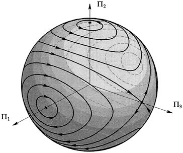
or can be verified directly from the Euler equations by computing the time derivative of

Because of conservation of

, the evolution in time of any initial point Π(0) is constrained to the sphere

. Thus we may view the Euler equations as describing a two-dimensional dynamical system on an invariant sphere. This sphere is called the reduced-phase space for the rigid body equations. Another constant of the motion is the Hamiltonian or energy:

. Since solutions curves are confined to the sets where H is constant, which are in general ellipsoids, as well as to the invariant spheres where

= constant, the intersection of these surfaces is precisely that of the trajectories of the rigid body, as shown in Figure 1.5.

Let us briefly indicate how geometric phases come into the rigid body example. Suppose we are given a trajectory Π(t) on P_μ that has period T and energy E. After time T the rigid body has rotated in physical 3-space about the axis μ by an angle given by

Here Λ is the solid angle enclosed by the curve Π(t) on the sphere and is oriented according to the right-hand rule, and k is an integer (reflecting the fact that we are really only interested in angles up to multiples of 2π).

FIGURE 1.5 The solutions of Euler's equations for rigid body motion.

An interesting feature of this formula is the fact that Δθ splits into two parts. The term A is the purely geometric quantity, the geometric phase. It does not depend on the energy of the system or the period of motion, but rather on the fraction of the surface area of the sphere that is enclosed by the trajectory. The second term, the dynamic phase, depends on the system's energy and the period of the trajectory.

Geometrically we can picture the rigid body as tracing out a path in its phase space; that is, the space of rotations (playing the role of positions) and corresponding momenta with the constraint of a fixed value of the spatial angular momentum. The phase space plays the role of the bundle, and the projection map to the base, the momentum sphere, is the map we described earlier that takes the orientation A and its velocity (or momentum) to the body momentum sphere. As Figure 1.5 shows, almost every trajectory on the momentum sphere is periodic, but this does not imply that the original curve of rotations was periodic, as is shown in Figure 1.6. The difference between the true trajectory and

a periodic trajectory is given by the geometric plus the dynamic phase. Although this figure is given in the context of rigid body dynamics, its essential features are true for any mechanical system with symmetry.

FIGURE 1.6 The geometric phase formula for rigid body motion.

This formula for the rigid body phase has a long and interesting history. It was known in classical books, such as that of Whittaker, in terms of quotients of theta functions, but not in terms of areas, as above. This aspect was discovered in the 1950s independently in work of Ishlinskii and of Goodman and Robinson. Montgomery (1991b,c) and Marsden et al. (1990) showed, following the lead of Berry and Hannay, that the formula can be interpreted in terms of holonomy of a connection. Further historical details may be found in Marsden and Ratiu (1994).

It is possible to observe some aspects of the geometric phase formula for a rigid body with a simple experiment. Put a rubber band around a book so that the cover will not open. (A tall thin book works best.) With the front cover facing up, gently toss the book in the air so that it rotates about its middle axis. Catch the book after a single rotation and you will find that it has also rotated by 180º about its long axis; that is, the front cover is now facing the floor.

In addition to its use in understanding phases, the mechanical connection has been helpful in stability theory. For example, when a rigid body such as a satellite tumbles about its long or short axis, it does so stably, but it is unstable when it rotates about the middle axis. When one takes into account small dissipative effects such as a vibrating antenna, then the rotational motion about the long axis becomes

unstable as well, but this effect is more delicate. Corresponding statements for systems like rigid bodies with flexible appendages or interconnected rigid bodies are more subtle than the dynamics of a single rigid body. There is a powerful method for determining the stability of such solutions called theenergy momentum method. This method is an outgrowth of basic work of Riemann, Poincaré, and others in the last century and more recently by Arnold; further recent developments were made by Simo et al. (1991), and Bloch et al. (1994, 1996) and references therein. Here the main problem is to split the variables properly into those that correspond to internal, or shape, changes, and to those that correspond to rotational and translational motions. Interestingly, the mechanical connection plays a key role in the solution of this problem and it makes many otherwise intractable problems soluble.

This gauge theory of mechanics has been successful for a number of important problems, such as the falling cat problem, as we shall discuss below. Nevertheless, there is another important class of problems that it does not apply to as stated, namely, mechanical systems with rolling constraints, typified by the constraint that a wheel or ball rolls without slipping on a plane. One very simple idea ties this type of problem to the zero angular momentum constraint problem that was just described. This idea is that of realizing the constraint as the horizontal space of a connection. In fact, the constraint itself defines a connection by declaring the constraint space to be the horizontal space. This, in effect, defines the connection. In the case of rolling constraints, we call this connection the kinematic connection to avoid confusion with the mechanical connection described earlier. This point of view for systems with rolling (and rolling type) constraints was developed by Koiller (1992) and by Bloch et al. (1997). For example, the equations of motion expressed on the base space again involve the curvature of the kinematic connection. This shows again that the links with geometry are strong at a very basic level.

Things get even more interesting when the system has both rolling constraints and symmetry. Then we have the kinematic connection as well as the symmetry group to deal with, but now they are interlinked. One of the things that makes systems with rolling constraints with symmetry different from free systems is that the law of conservation of angular momentum is no longer valid for them. This is already well illustrated by a toy called the rattleback, a canoe-shaped piece of wood or plastic. When the rattleback rocks on a flat surface like a table, the rocking motion induces a rotational motion, so that it can go from zero to nonzero angular momentum about the vertical axis as a result of the interaction of the rocking and rotational motion and the rolling constraint with the table. One can say that the forces of constraint that enforce the condition of rolling can upset the balance of angular momentum. This is also the case for the snakeboard discussed below, but nonetheless, this rams out to be a key point in understanding locomotion generation for this system. One of the interesting aspects of this is that, as shown by Bloch et al. (1996), there is a very nice equation satisfied by a particular combination of the linear and angular momentum, which they call the momentum equation. Because of that success, one can imagine that this understanding will be important for many other similar systems as well.

↧

STABILIZATION AND OPTIMAL CONTROL

September 14, 2018, 4:11 am

≫ Next: THE SNAKEBOARD

≪ Previous: CONSTRAINTS: ANGULAR MOMENTUM AND ROLLING

Control theory is closely tied to dynamical systems theory in the following way. Dynamical systems theory deals with the time evolution of systems by writing the state of the system, say z in a general space P, and writing an evolution equation

for the motion, where μ includes other parameters of the system (masses, lengths of pendula, etc.). The equations themselves include things like Newton's second law, the Hodgkin-Huxley equations for the propagation of nerve impulses, and Maxwell's equations for electrodynamics, among others. Many valuable concepts have developed around this idea, such as stability, instability, and chaotic solutions.

Control theory adds to this the idea that in many instances, one can directly intervene in the dynamics rather than passively watching it. For example, while Newton's equations govern the dynamics of a satellite, we can intervene in these dynamics by controlling the onboard gyroscopes. One simple way to describe this mathematically is by making f dependent on additional control variables u that can be functions of t, z, and μ. Now the equation becomes

and the objective, naively stated, is with an appropriate dependence of f on uto choose the function u itself to achieve certain desired goals. Control engineers are frequently tempted to overwhelm the intrinsic dynamics of a system with the control. However, in many circumstances (fluid control is an example—see, for example, the discussion in Bloch and Marsden, 1989), one needs to work with the intrinsic dynamics and make use of its structure.

Two of the basic notions in control theory involve steering and stabilizability. Steering has, as its objective, the production of a control that has the effect of joining two points by means of a solution. One imagines manipulating the control, much the way one imagines driving a car so that the desired destination is attained. This type of question has been the subject of extensive study and many important and basic questions have been solved. For example, two of the main themes that have developed are, first, the Lie algebraic techniques based on brackets of vector fields (in driving a car, you can repeatedly make two alternating steering motions to produce a motion in a third direction) and, second, the application of differential systems (a subject invented by Elie Cartan in the mid-1920s whose power is only now being significantly tapped in control theory). The work of Tilbury et al. (1993) and Walsh and Bushnell (1993) typify some of the recent applications of these ideas.

The problem of stabilizability has also received much attention. Here the goal is to take a dynamic motion that might be unstable if left to itself but that can be made stable through intervention. A famous example is the F-15 fighter, which can fly in an unstable (forward wing swept) mode but which is stabilized through delicate control. Flying in this mode has the advantage that one can execute tight turns with rather little effort—just appropriately remove the controls! The situation is really not much different from what people do everyday when they ride a bicycle. One of the interesting things is that the subjects that have come before—namely, the use of connections in stability theory—an be turned around to be used to find useful stabilizing controls, for example, how to control the onboard gyroscopes in a spacecraft to stabilize the otherwise unstable motion about the middle axis of a rigid body (see Bloch et al., 1992; Kammer and Gray, 1993).

Another issue of importance in control theory is that of optimal control. Here one has a cost function (think of how much you have to pay to have a motion occur in a certain way). The question is

not just if one can achieve a given motion but how to achieve it with the least cost. There are many well-developed tools to attack this question, the best known of these being what is called the Pontryagin Maximum Principle. In the context of problems like the falling cat, a remarkable consequence of the Maximum Principle is that, relative to an appropriate cost function, the optimal trajectory in the base space is a trajectory of a Yang-Mills particle. The equations for a Yang-Mills particle are a generalization of the classical Lorentz equations for a particle with charge e in a magnetic field B:

where v is the velocity of the particle and where c is the velocity of light. The mechanical connection comes into play though the general formula for the curvature of a connection; this formula is a generalization of the formula

expressing the magnetic field as the curl of the magnetic potential. This remarkable link between optimal control and the motion of a Yang-Mills particle is due to Montgomery (1990, 1991a).

One would like to make use of results like this for systems with rolling constraints as well. For example, one can (probably naively, but hopefully constructively) ask what is the precise connection between the techniques of steering by sinusoids mentioned earlier and the fact that a particle in a constant magnetic field also moves by sinusoids, that is, moves in circles. Of course if one can understand this, it immediately suggests generalizations by using Montgomery's work. This is just one of many interesting theoretical things that requires more investigation. One of the positive things that has already been achieved by these ideas is the beginning of a deeper understanding of the links between mechanical systems with angular momentum type constraints and those with rolling constraints. The use of connections has been one of the valuable tools in this endeavor. One of the papers that has been developing this point of view is that of Bloch et al. (1997). We shall see some further glimpses into that point of view in the next section.

↧

THE SNAKEBOARD

September 14, 2018, 4:13 am

≫ Next: AR/VR Display Technology Roundup: OLEDs, GaN-on-Silicon, and Foveated Rendering

≪ Previous: STABILIZATION AND OPTIMAL CONTROL

The snakeboard is an interesting example that illustrates several of the ideas we have been discussing (see Lewis et al., 1997). This device is a modification of the standard skateboard, the most important of which is that riders can use their feet to independently turn the front and back wheels—in the standard skateboard, these wheels are of course fixed to the frame of the skateboard. In addition, one can manipulate one's body using a swivelling motion and this motion is coupled to the motion of the snakeboard itself. We show the snakeboard schematically in Figure 1.7.

One of the fascinating things about the snakeboard is that one can generate locomotion without pedaling, solely by means of internal motions. When the user's feet and body are moved in the right way, rotational and translational motion of the device can be generated. The snakeboard is simple enough that one can study many parts of it analytically and numerical simulations of its motion are reasonably economical to implement. On the other hand, it seems to have all of the essential features that one would want for more complex systems, the main one for the present goals being its ability to generate rotational and translational motion. From the mathematical and mechanical point of view, it is rich in geometry and in symmetry structure, which also makes it attractive. Thus, it provides a good testing and development ground for both theoretical and numerical investigations.

From the theoretical point of view, one feature of the snakeboard that sets it truly apart from examples like the planar skater and the falling cat is that even though it has the symmetry group of rotations and translations of the plane, the linear and angular momentum is not conserved. Recall that for the planar skater, no matter what motions the arms of the device make, the values of the linear and angular momentum cannot be altered. This is not true for the snakeboard and this can be traced to the presence of the forces of constraint, just as in the rattleback mentioned earlier. Thus, one might suspect that one should abandon the ideas of linear and angular momentum for the snakeboard.

However, a deeper inspection shows that this is not the case. In fact, one finds that there is a special component of the angular momentum, namely that about the point P shown in Figure 1.8.

If we call this component p, one finds that, due to the translational and rotational invariance of the whole system, there is a ''momentum equation'' for p of the form

FIGURE 1.7 The snakeboard has three movable internal parts, the front and back wheels and the angle of the rider's body.

where x represents the internal variables of the system (the three angles shown in the preceding figure). The point is that this equation does not depend on the rotational and translational position of the system. Thus, if one has a given internal motion, this equation can be solved for p and, from it, the attitude and position of the snakeboard calculated by means of another integration. This strategy is thus parallel to that for the falling cat and the planar skater.

With this set-up, one is now in a good position to identify the resulting geometric phase with the holonomy of a connection that is a synthesis of the kinematic and mechanical connection. Carrying this out and implementing these ideas for more complex systems is in fact the subject of current research.

FIGURE 1.8 The angular momentum about the point P plays an important role in the analysis of the snakeboard.

ACKNOWLEDGMENTS

Thanks are extended to John Tucker, Tony Bloch, Roger Brockett, Joel Burdick, P.S. Krishnaprasad, Andrew Lewis, Richard Montgomery, Richard Murray, Jim Ostrowski, Tudor Ratiu, Shankar Sastry, Greg Walsh, and Jeff Wentlandt for their kind advice and help.

↧

AR/VR Display Technology Roundup: OLEDs, GaN-on-Silicon, and Foveated Rendering

September 14, 2018, 4:17 am

≫ Next: VIDEO:Mpambano kati ya Sam Eggington vs Hassan Mwakinyo

≪ Previous: THE SNAKEBOARD

Here’s a snapshot of where our display technology is at right now—and a little bit of what is just around the corner.

The virtual and augmented reality immersive experience is heavily influenced by the display technology behind it.

If a display is too heavy, doesn’t have a high enough resolution, requires too much power, or doesn’t provide a sufficient field of view, the illusion isn’t quite as good, or the useful application of the display could be diminished.

This past May, the International Development Corp (IDC) released a report in which it forecasted that $27 billion USD would be spent on VR/AR in 2018, which is a 92% growth compared to 2017. This number is expected to eventually reach $53 billion USD by 2023.

This growth certainly incentivizes the improvement of display technology, whether it is being used for industrial or leisure purposes.

Here’s a snapshot of where our display technology is at right now, and a little bit of what is just around the corner.

Recreating Human Vision: 1443 ppi OLED

Google and LG have been collaborating on R&D efforts to develop a head-mounted display that recreates natural human vision as closely as possible. The specs needed to achieve this include a field of view (FoV) that is 160 degrees (horizontal) by 150 degrees (vertical), and has a per eye resolution of 9600x9000 pixels for 20/20 acuity.

In a paper published in the Journal of the Society for Information Display, the challenges in achieving these specs are discussed. Two of the biggest challenges come from the required pixel pitch to achieve human vision acuity, as well as the refresh rate required.

First, the pixel pitch; this describes the distance between pixel clusters and determines the optimal viewing range for a given resolution. To recreate human vision acuity, this optimal distance would vary across the display. This would add a considerable amount of complexity in the design, and so instead a uniform pixel pitch was calculated at 11.4 µm, which would require a 4.3 display with 2138 ppi for a 160-degree FoV.

For the refresh rate, the line time to refresh a row of pixels would be only 694 µs and require a pixel clock of 14.3 GHz

Achieving these specs would be incredibly difficult and they still wouldn't be able to produce usable results since they would require heavy lenses, complicated circuitry, etc. Therefore, a balance of trade-offs was needed and the end result is a 4.3-inch display, providing a 100 degree (horizontal) by 96 degree (vertical) FoV, 17.6 µm pixel pitch, and 1443 ppi. The display is driven using an n-type LTPS TFT backplane to reduce ghost image artifacts, with the video stream is converted for the display using an FPGA.

The experimental display is reported to be the highest resolution OLED currently developed.

An example rendering from the experimental OLED using foveated rendering. Image courtesy of Journal of the Society for Information Display.

Monolithic MicroLED on GaN-on-Silicon Wafers

Plessey Semiconductors and Jasper Display Corp (JDC) announced a partnership in the development of a monolithic microLED using GaN-on-Silicon wafers and JDC’s eSP70 silicon backplane.

GaN-on-silicon uses gallium nitride in a silicon substrate as a semiconductor. This material has the advantages of being thermally efficient, an excellent optical emitting surface, and a lower efficiency drop in light emission when scaled. It first showed potential in RF and microwave applications but is expected to become more mainstream over time in other applications as the advantages are realized.

GaN-on-Silicon wafer. Image courtesy of Plessey Semiconductors.

These combined properties reduce the power requirements for bright images on LED displays. The eSP70 backplane can provide a 1920x1080 resolution at a pixel pitch of 8µm, and will be paired with Plessey’s microLED on a GaN-on-Silicon wafer.

The companies are specifically targeting VR/AR applications with low power, low cost, and small form factor displays.

Foveated Rendering

Foveated rendering, while maybe not hardware-based in itself, is still an important part of improving display technology for VR/AR. The technique’s name comes from the part of the eye called the fovea centralis—the part of the eye responsible for focused vision, such as when we are reading.

In foveated rendering, eye tracking technology is used in combination with the VR/AR head mounted display to determine where in the image the user is focusing their gaze. Based on that, the system will render parts of the image most immediate in the user’s foveal viewing range more sharply and gradually soften further into the peripheral viewing range.

This helps overcome the hardware challenges for rendering a high-resolution image stream and lowers the workload on the GPU or other specialized hardware.

Foveal rendering was first demonstrated at CES 2016 by SensoMotoric Instruments and Omnivision. Since then, it has been adopted by NVIDIA, Google, LG, with others surely following the lead.

What other AR/VR display technologies have caught your eye recently?

↧

VIDEO:Mpambano kati ya Sam Eggington vs Hassan Mwakinyo

September 14, 2018, 9:51 am

≫ Next: Hands on: iPhone XS Max review

≪ Previous: AR/VR Display Technology Roundup: OLEDs, GaN-on-Silicon, and Foveated Rendering

The Arena Birmingham was stunned as Sam Eggington suffered a shock defeat to Hassan Mwakinyofro Tanzania Tanga

↧

Hands on: iPhone XS Max review

September 14, 2018, 12:19 pm

≫ Next: Why Do We Need Matched Termination with High Speed Logic Families?

≪ Previous: VIDEO:Mpambano kati ya Sam Eggington vs Hassan Mwakinyo

The phone for those who want it all

OUR EARLY VERDICT

The iPhone XS Max appears to be the perfect upgrade for owners of the iPhone Plus who prefer a large form factor with a big screen and a bigger battery. It packs in all the top-end features of the smaller model, but really turbocharges them in the hand.

FOR

Big and beautiful screen
Good battery life
Improved camera

AGAINST

Two-handed device
Even more expensive

Get ready for an all-new breed of iPhone - this is the iPhone XS Max. That's the iPhone 'Ten S' Max, not the 'Excess Max', but that's what most people will be seeing in this name. That would miss out on what's an interesting new product, especially for iPhone fans.

It has a massive 6.5-inch screen along with a bigger battery, plus all the other features present in the smaller iPhone XS such as dual SIM support, an improved camera setup and the super-fast A12 Bionic processor and a new 512GB storage option.

Update: iPhone XS Max pre-orders are now open!

Although in the past Apple has differentiated the Plus models with a better camera setup, the iPhone XS Max is identical to the iPhone XS other than the larger screen and battery.

What's the difference between the three new iPhones? Watch our handy explainer below:

Below you'll find links to all of our other iPhone and Apple hands on reviews from the big event...

iPhone XS Max price and release date

The iPhone XS Max, along with the iPhone XS, pre-orders in most countries around the world are now open, and will go on sale from September 21.

It'll be available in 64GB, 256GB and 512GB configurations, and it'll be Apple's most expensive phone to date – although that was expected after Apple introduced the only slightly less expensive iPhone X last year.

On average, the iPhone XS Max price is about $100 / £100 more expensive than the smaller iPhone XS, with the 64GB model priced at at $1,099 / £1,099 / AU$1,799 / AED4,649. The 256GB price is $1,249 / £1,249 / AU$2,049/ AED5,279 while the most expensive 512GB version will set you back $1,449 / £1,449 / AU$2,369 / AED6,129.

That makes the iPhone XS Max the most expensive 'regular' handset on the market, with only special editions such as the Huawei Porsche Design costing more.

Design

The iPhone XS Max measures 157.5 x 77.4 x 7.7mm, which puts it around the same size as the Samsung Galaxy Note 9, which comes in at 161.9 x 76.4 x 8.8mm. This is a big phone, and there's no way you'll be able to use it with one hand.

Interestingly, even though the iPhone XS Max is slightly heavier than the Galaxy Note 9 (208 grams vs 202 grams), in the hand it feels lighter than its rival. In other words, the iPhone XS Max looks like a big and heavy device, but you'll be pleasantly surprised when you pick it up.

Like other iPhone X models, the iPhone XS Max is basically two slabs of glass with a stainless steel frame joining them.

IPHONE XS MAX SPECS

Weight: 208g
Dimensions: 157.5 x 77.4 x 7.7mm
OS: iOS 12
Screen size: 6.5-inch
Resolution: 2688 x 1242
CPU: A12 Bionic
Storage: 64/256/512GB
Rear camera: 12MP + 12MP
Front camera: 7MP
Colors: Silver, Space Grey, Gold
Resistance: IP68

Apple claims that it has used the most durable glass ever made for a smartphone, and it felt less slippery than we expected – but it is a big glass device at the end of the day, and we recommend getting a cover for it if you're spending all that money on one.

The new iPhone XS and XS Max are now rated at IP68, which means they're water-resistant for up to two meters and 30 minutes. Apple says it has tested these new phones by submerging them in fresh water, salt water and various other liquids – including beer – to make sure they come out unharmed.

The button and port configuration on the iPhone XS Max is the same as on the smaller model, with the volume buttons and the silence switch on the left, and the power button and SIM card tray on the right.

Apple is bringing dual-SIM functionality to its iPhones for the first time, with the new handsets able to support eSIM in addition to having a nano SIM slot. eSIM means 'embedded SIM', and it's a piece of hardware which acts like a SIM card but saves you having to physically swap cards – instead you download software to the phone to change your plan or carrier.

You'll use a QR code to upgrade it, and in the future apps may be developed where you can download it from a carrier and sign up from within it - although that won't be around for a while.

The iPhone XS Max will be available in three color options: space grey and silver make a return, with a new gold version that looks pretty impressive, especially with the golden stainless steel band around it.

Screen

The biggest draw for anyone thinking about the iPhone XS Max will be the OLED screen, and it's simply stunning on Apple's largest phone. It's gigantic at 6.5 inches, and provides quite the immersive experience, especially with movies and games – provided you can overlook the notch.

Yes, the notch is still present on the iPhone XS Max, although because of the larger screen you have more screen to the left and right of the notch than on the iPhone X.

That being said, we've been using the iPhone X for almost a year now and we don't really think about the notch anymore; you learn to live with it, and before long it just disappears into the background, although that may not be your experience initially.

Specs-wise, the OLED panel on the iPhone XS Max has a resolution of 2688 x 1242 pixels, giving it the same density as the smaller iPhone XS at 458ppi. Apps can now work in split mode, much like they do on the Plus versions of previous iPhones.

We're not sure if third-party apps will be able to use the new resolution right away though, or whether developers will need to update their apps to support the new resolution.

As on the iPhone X the screen supports TrueTone technology as well as 120Hz input. We were hoping the XS Max would support the True Motion technology found on the iPad Pro, which makes scrolling and moving within the UI very fluid, but that's not the case.

Apple claims the screen now has a 60% better dynamic range, which should make your photos and videos appear more vivid. We tried the new Bethesda game The Elder Scrolls: Blades, and visually it looked very appealing, although we did notice some stuttering as we flicked around the gameplay settings.

Camera

The camera on the iPhone XS Max is similar to the one on last year's iPhone X, with a dual lens setup, however, Apple has made improvements to both the hardware and software.

You're still getting two 12MP sensors on the back, but the pixel size has now been increased to 1.4um on the wide-angle camera. The secondary 12MP camera is still fixed at 2x zoom levels with an f/2.4 aperture and OIS.

Meanwhile Apple has improved its camera software by introducing a new Smart HDR mode with zero shutter lag. This allows the iPhone to capture multiple images, and, by teaming the camera sensor with the AI neural processing unit, select and combine the best bits from each frame to produce a single perfectly exposed image.

It's a similar process to that used on some Android phones, like the Google Pixel 2 and the Huawei P20 Pro.

Another new software feature is the ability to change the depth of field – that is, which parts of the image are in focus or creatively blurred – after you've taken a picture.

Apple claims this is slightly different to the rest of the competition that offers the capability to alter the background blur post-snap because it actively changes the exposure - thus resulting in a more natural image.

Battery

As well as the larger screen, the iPhone XS Max also has the largest battery Apple has ever put in an iPhone. We don't know the capacity yet, but Apple is promising an extra 90 minutes of battery life over the iPhone X.

It also packs wireless charging capabilities like recent iPhones have added in, based on the Qi standard - although sadly there's no fast charger in the box as was previously rumored.

We'll be making sure to give the battery a full workout when we get our hands on the new iPhones for our full reviews. The Plus versions of previous iPhones have had killer battery life, so we have high hopes for the iPhone XS Max.

Early verdict

The iPhone XS Max is clearly aimed at fans of the Plus-size iPhones – those who want a large device with a large screen, and a large battery to go with it.

It's very close in size to the Plus models, so if you're comfortable with one of those phones – and this is strictly a two-handed device – you'll feel right at home with the iPhone XS Max.

With dual SIM capabilities, an updated camera module and the new, super-fast A12 Bionic processor, Apple looks to be on track to deliver its best iPhone yet.

If you can get over the size and price (and that’s a big ask) the iPhone XS Max is the phone to go for out of the three new devices, packing in the best of everything Apple showcased at its launch event.

We come back to the above points about size and price though: this is a gargantuan phone in every way, and we’re looking forward to putting it through its paces to find out whether it’s just an oversized version of the iPhone XS, or the supercharged, super-sized iPhone you’ll want to go for.

WHAT IS A HANDS ON REVIEW?

'Hands on reviews' are a journalist's first impressions of a piece of kit based on spending some time with it. It may be just a few moments, or a few hours. The important thing is we have been able to play with it ourselves and can give you some sense of what it's like to use, even if it's only an embryonic view.

↧

Why Do We Need Matched Termination with High Speed Logic Families?

September 15, 2018, 8:51 am

≫ Next: How to Design a Super Simple Sensor System for Industrial Monitoring Applications

≪ Previous: Hands on: iPhone XS Max review

This article will try to develop a better insight into wave reflection that can occur when driving a relatively long wire with a fast logic gate.

Delay of Wires

An electrical signal has a finite speed when travelling through a wire. The exact value of the speed depends on the characteristics of the wire, but we can assume a speed of about half the speed of light, which is nearly

\frac{1}{2} \times 3 \times 10^{8}

m/s. Therefore, an electrical signal needs about 1 nanosecond (ns) to propagate through a 15 centimeter (cm) wire.

The Signal Rise and Fall Time

Now, assume that we have a fast logic family which exhibits rise and fall times of about 1 ns. What happens if we connect this high speed logic to a relatively long wire that introduces a delay comparable to the signal rise time?

As you may have guessed, in such cases, we may not be able to treat the wire as an ideal zero-delay conductor. In fact, the logic gate may apply a voltage transition to the beginning of the wire while the other end of the wire still has its previous voltage value. Can this phenomenon give us trouble? We’ll answer this question later in the article. First we’ll discuss transmission lines.

Transmission Lines

When we’re working with high-speed signals, we often need to think in terms of transmission lines instead of ordinary wires. Transmission lines require special analysis techniques, and they are implemented with greater attention to such details as the distance between a conductor and a ground shield or the dimensions of a PCB trace. A transmission line can be modeled as follows:

Figure 1. Click to enlarge.

The transmission line is divided into smaller sections, and each section is modeled using some passive elements. As shown in the figure, these passive components are distributed along the wire. Here, R and G represent, respectively, the resistance of the wire and the conductance of the dielectric that separates the conductors. L and C represent the inductance and the capacitance of the transmission line.

Note that generally the distributed element model for a transmission line uses an infinite series of cells as shown in Figure 2 below.

Figure 2. Cell schematic used to model a transmission line. Image courtesy of Omegatron [CC BY-SA 3.0]

In Figure 2, the value of the components R, L, G, and C are specified per unit length. However, in our model shown in Figure 1, the value of the components are not per unit length. In Figure 1, we assume that a given length of the transmission line is divided into sufficiently small segments (or, equivalently, n is sufficiently large), so that each segment can be represented by some passive components. Using this model, we'll provide an intuitive understanding of the electrical wave reflection in a transmission line. To simplify this article’s discussion, we'll assume that the wire is lossless (R = G = 0). This will give the model shown in Figure 3.

Figure 3. Click to enlarge.

As mentioned above, we intend to develop an intuitive understanding of the reflection phenomenon based on the circuit model of a lossless transmission line. While the overall shape of the waveforms given below can be verified by circuit simulations, there can be differences between the waveforms obtained from a circuit simulator (examples are given at the end of the article) and the simplified plots provided in the more theoretical discussion of this topic. However, the main goal of this article is not discussing the exact waveforms; instead, we want to explain electrical wave reflection by replacing a transmission line with its circuit model.

Now, let’s use the model in Figure 3 to examine connecting a high-speed logic gate to a wire that is long with respect to the signal rise time.

A Transmission Line of Infinite Length

First, assume that the gate is connected to a transmission line of infinite length. Figure 4 shows a model for the low-to-high transition. In this figure, Rs is the output impedance of the gate when going from logic low to logic high and Vs is the logic-high voltage. In this article, we’ll assume that the output resistance of the gate, Rs, is equal to

\sqrt{\frac{L}{C}}

. The reason for this assumption will be explained at the end of the article.

Figure 4. Click to enlarge.

In Figure 4, we have assumed a very abrupt transition from low to high. The figure shows that the cells that are farther along the wire experience a larger delay, i.e.,

t_{3}

t_{2}

t_{1}

. Also, note that while the input source applies a transition from 0 to Vs, the voltage transitions of the cells are from zero to kVs! The factor k is less than one; we won’t go through the mathematics needed to derive the exact value.

We have assumed that the line is of infinite length. Thus, there is always a cell along the wire that hasn’t experienced the voltage transition yet. The current that causes the transition for this particular cell must be supplied by the voltage source placed at the beginning of the wire. This current will have to flow through the cells that are closer to the source, and eventually it will be delivered to the cell experiencing the voltage transition. Since the current is flowing from the source toward the wire, we can conclude that the voltage developed across the cells is less than Vs(i.e., k<1 p="">

It can be shown that the factor k is equal to

\frac{Z_{0}}{Z_{0} + R_{S}}

, where

Z_{0}

is the characteristic impedance of the transmission line. The characteristic impedance is determined by the geometry and materials of the transmission line and, for a uniform line, is not dependent on its length. Refer to the textbook page on transmission lines in the AAC RF textbook for more details.

A Short-Circuited Transmission Line

Now that we’re familiar with an electrical wave propagating through a wire of infinite length, let’s examine the propagation along a short-circuited transmission line, as shown in Figure 5. To simplify our discussion, we are showing only four cells in the figure.

Figure 5. Click to enlarge.

The figure presents the waveforms for

t < T

, where T is the delay from the beginning of the transmission line to its far end, which is short-circuited by the red wire. For

t < T

, the waveforms of Figure 5 and 4 are the same. In fact, in this interval, the short-circuit forces zero voltage across the fourth cell of Figure 5 but note that this voltage was initially assumed to be zero in Figure 4.

However, for

t > T

, the two circuits exhibit different behavior. In Figure 5, the output of the fourth cell is forced to remain at zero volts. The short circuit actually provides a path for discharging the previous cells too. That’s why after some delay

V_{3}

will exhibit a transition to zero. This will in turn cause

V_{2}

to go to zero after some delay. Hence, we obtain the final waveforms as shown in Figure 6.

Figure 6. Click to enlarge.

An Open-Circuited Transmission Line

Now, let’s examine the electrical wave propagation along an open-circuited transmission line as shown in Figure 7. Again, to simplify our discussion, we are showing only four cells in the figure.

Figure 7. Click to enlarge.

The figure also depicts the waveforms for tT, the circuit shows a different behavior. Since there isn’t any other cell after the fourth cell, the final cell will be able to charge to Vs rather than kVs. Now that the fourth cell is charged to the source voltage, the current flowing into this cell will tend to zero. This will allow the third cell to charge up to Vs. Then, the voltage across the other cells that are closer to the source will reach Vs in a similar manner. Note that the cells that are closer to the end of the transmission line will experience a shorter delay to reach their final value. The complete waveforms will be as shown in Figure 8.

Figure 8. Click to enlarge.

Reflection Coefficient

To have a unified treatment of the problem, we can define a reflection coefficient:

ρ = \frac{Z_{t e r m} - Z_{0}}{Z_{t e r m} + Z_{0}}

Where

Z_{t e r m}

and

Z_{0}

are the termination impedance and the characteristic impedance of the transmission line. For example, consider the waveforms shown in Figure 6. In this case, the termination impedance is zero which gives

ρ = - 1

. This means that the original waveform shown in Figure 5 will be reflected with a reflection coefficient of -1. In other words, a wave with magnitude equal to the original wave but with the opposite polarity will be reflected from the short-circuited end of the transmission line.

For the waveforms of Figure 8, the terminating impedance is infinity which gives

ρ = 1

. Hence, a wave equal to the original wave will be reflected from the open-circuited end of the transmission line. Adding the reflected waveform to the original waveform leads to the waveforms shown in Figure 8.

Avoiding Reflections

The above discussion shows the importance of the resistance that terminates a transmission line. As you can see from the examples, different termination resistances lead to different reflection coefficients. How can we avoid reflections?

We observed that there’s no reflection when the transmission line is of infinite length. In practice, we cannot have a transmission line with infinite length, but we can use a termination resistance equal to the characteristic impedance of the line to avoid reflections. This can be also verified using Equation 1 which gives

ρ = 0

for

Z_{t e r m} = Z_{0}

. For example, when positive-referenced emitter-coupled logic (PECL) is driving a load through a transmission line, we terminate the transmission line to a resistance close to the characteristic impedance of the line. This is shown in Figure 9.

Figure 9. Thevenin termination for a PECL gate driving a 50 transmission line. Image courtesy of idt.

In the example of Figure 9, the termination resistance is

R_{1} | | R_{2} = 50 Ω

which is equal to the characteristic impedance of the line. It’s worthwhile to note that, in addition to providing a matched termination, the values of the resistors determine the DC level for the input of the PECL receiver. In this example, the resistors are chosen to set the DC level of the inputs to about 1.3V.

In the above examples, we saw that the end of the transmission line can reflect the propagating wave when

Z_{t e r m}

is not equal to

Z_{0}

. It should be noted that the reflected wave itself can be re-reflected when reaching the beginning of the transmission line if the source resistance, Rs, is not equal to

Z_{0}

. Since the characteristic impedance of a lossless transmission line is equal to

\sqrt{\frac{L}{C}}

, we assumed

R s = \sqrt{\frac{L}{C}}

at the beginning of the article to avoid re-reflection of the reflected waves.

If the rise time of the logic gate is longer than 2T, where T is the delay of the wire, then we can ignore the reflections. In this case, the reflections return while the input is still rising, so we’ll have a somewhat slowed and “bumpy” rising edge but the overall functionality will be fine.

Some Simulations

In previous sections, we used a circuit model to examine electrical wave reflection along a transmission line. Now, we’ll look at some waveforms obtained from circuit simulations. In these simulations, we have cascaded 20 LC cells to model a hypothetical transmission line. Similar to the schematic shown in Figure 5, the end of the transmission line is short-circuited. A low to high transition is applied to the beginning of this transmission line. In the first simulation waveform shown in Figure 10, we have chosen L = 2.5 nH and C = 1 pF. In this figure, the red curve is the pulse applied to the input of the transmission line and the blue curve is the voltage observed at the output of the 10th cell. As you can see, at first, we have a transition from low to high. Then, after some delay, the waveforms exhibit a transition from high back to low. This is consistent with the waveforms we obtained for Figure 5. However, unlike the waveforms of Figure 5, we have some ringing behavior in Figure 10.

Figure 11. Simulation waveforms for a short-circuited transmission line model with L = 2.5 nH and C = 1 pF. Click to enlarge.

Now, we will change the value of L and C to 0.05 nH and 0.02 pF. In this case, the waveforms are as shown in Figure 11.

Figure 11. Simulation waveforms for a short-circuited transmission line model with L = 0.05 nH and C = 0.02 pF. Click to enlarge.

Comparing Figure 10 with Figure 11, we observe that there may or may not be ringing effect but the overall behavior is as discussed in the article: with a short-circuited line at the far end, the voltage waveforms return to zero volts due to the wave reflection phenomenon. Why do you think the value of L and C can affect the ringing behavior of the waveforms? If you have any explanation for this phenomenon, feel free to share it with us in the comments below.

To see a complete list of my articles, please visit this page.

↧

How to Design a Super Simple Sensor System for Industrial Monitoring Applications

September 15, 2018, 8:55 am

≫ Next: AR/VR Display Technology Roundup: OLEDs, GaN-on-Silicon, and Foveated Rendering

≪ Previous: Why Do We Need Matched Termination with High Speed Logic Families?

This article describes an Ethernet-connected subsystem of a larger modular sensor system designed for industrial or smart home sensing and monitoring. We will discuss a custom sensor subsystem developed for this application.

Creating custom sensor solutions for home or automation typically requires a great deal of customization. A variety of sensors from perhaps several manufacturers are collected on a circuit board, firmware must be engineered, and a user interface or dashboard created. It isn’t overwhelmingly difficult work—but it can be rather tedious and time-consuming. The customization aspect may also make it cost-prohibitive in many use cases.

The idea behind this project was to create a “Super Simple Sensor System” that allows a wide variety of input and output nodes to be linked together with a common protocol with the fewest number of wires possible and low upgrade/replacement cost. This subsystem will hopefully spark creativity in your designs but it is not a market-ready product.

The inspiration came from the wonderfully designed Makeblock Neuron line of children’s educational toys. Multiple sensors and inputs (temperature, humidity, joystick, buttons, etc.) are connected with a variety of outputs and interfaces (LED display, buzzer, etc.) and all of the devices connect via magnetic spring-loaded pogo-pin connectors.

Project overview: Each node connects to its neighboring node with power, ground, and two UART connections. Click to enlarge.

Choosing a Communication Protocol

Each node in my project has an inexpensive microcontroller built in. Sensor or mechanical input data is sent to the microcontroller through the interface appropriate for the sensor (SPI, I2C, CAN, 4-20mA, etc.) and the microcontroller then converts the data to a common interface (UART, USB, etc.) for transmission to neighboring nodes.

In this case, I chose UART as the common bus protocol. Data is read from the neighboring node on the left, data from the current sensor is added to the stream, and then all of the data is passed to the neighboring node on the right.

Each input node adds to the datastream, perhaps with a byte identifying data length, a node identification byte, and the data. Designers who wish to augment the system need only design a single node; this retains modularity of design and allows a catalog of devices to be connected quickly and easily.

Data is continually passed in daisy-chain fashion from one node to the next until it reaches an output node. There the output devices (flashing alarms, LCD displays, buzzers, etc.) read the datastream for information that pertains to them and act accordingly—passing the data along the entire time.

This would work well enough for a three-wire interface (VDD, GND, Data) with one UART bus, but would require that all input nodes be placed before output nodes. By adding a second UART bus, bidirectional information can be passed and nodes can be added in any configuration. Alternatively, the second line might be used for microcontroller software updates, as a heartbeat monitor, or reserved for future use.

You can make life easier by using magnetic pogo-pin connectors in your design.

Image of magnetic pogo pin connectors courtesy of Shenzhen Like Hardware Electronics, Co. LTD.

As indicated above in the block diagram, the Tx/Rx lines (for both UART0 and UART1) extend to opposite sides of the board. This is for several reasons.

First, and perhaps most important, this allows simultaneous programming/debugging and use. The microcontroller programming interface shares pins with UART0 (i.e., the programming signal and the UART signal are both routed to the same physical pin), so testing a receive and transmit sequence, which happens on opposite sides of the board, while connected to the debugger, requires that one of the two data pins from UART1 be on either side of the board.

Second, it allows a single UART bus to be utilized in a three-wire configuration (i.e., power, ground, Tx on one side and power, ground, Rx on the other side).

Lastly, it might simplify the firmware by allowing data to be received and transmitted using the same bus instead of being copied from a receive bus to a separate transmit bus each time it enters a node.

Designing with Industrial Communications in Mind: About the Subsystem

Sensors and displays on a factory floor tend to be ignored over time. Data must be moved from the factory floor to a central location in the building, or perhaps across town to a monitoring location. To satisfy that requirement, I chose to use a wired Ethernet connection. Cat5 and Cat6 wiring, usually already installed at a location, can transmit data over long distances in a LAN, and when connected to WAN, can move data anywhere in the world. The MQTT protocol is designed for M2M (machine-to-machine) communication, and an MQTT broker can easily be established to move the data from interface node to interface node, all the while being secured withTLS1.3.

Once the data reaches its destination in the LAN, or the Internet, a programmer can capture the data to create a graphical user interface, sometimes referred to as a “dashboard,” that managers and controllers can view. Unfortunately, those displays tend to gradually be ignored over time as well. The current trend in automation is to create automated texts, emails, or other alerts that can be sent directly to workers, and then if the worker does not correct the errant situation in a timely fashion, notify the employee’s direct supervisor.

The critical parts of this project require that I have two independent UART buses and one Ethernet interface. For the Ethernet interface, I chose the WizNET W5500. This highly integrated IC implements the TCP/IP stack, the 10/100 Ethernet MAC (media access control), and the PHY (physical layer). I don’t have much experience with the TCP/IP stack, UDP, ARP, ICMP, etc., and this IC allows me to use up to 8 sockets over SPI—a protocol I am familiar with.

I selected the MSP430FR2633 as the microcontroller. While the MSP430FR2433 would also be able to control the W5500, I knew I would have some unused GPIO pins, and I liked the option of creating a low-costcapacitive-touch control panel in the future. The 2433 does not support capacitive touch, so I opted for the 2633. All other ICs used in the project support the W5500 and the MSP430FR2633.

Power

Each node in the system shares a common 5VDC rail. The 5V supply is generated by one board that serves as the power source for the entire network, and then each board uses two TLV757P LDOs to regulate the 5V rail to 3.3V for analog circuitry and 3.3V for digital circuitry. This is a four-layer board, with the top and bottom layers used for signals and layers 2 and 3 for AVDD and GND, respectively.

The schematic diagram of the power section

Routing of the AVDD and DVDD lines provided a challenge on this 4-layer board. AVDD (shown in magenta below) was chosen as the power-plane net because this arrangement seemed to result in easier, cleaner routing. DVDD had to move between layers 1, 2, and 4, which is not ideal. At each transition, multiple vias were used to minimize the impedance.

Shown above is the physical PCB, followed by layers 1-4 of the layout. Layer 2 (AVDD) is shown in magenta, and DVDD is shown in orange.

Ethernet Connectivity

Almost all devices that are hard-wired to the Internet have an 8P8C RJ45 jack. Either built into the jack or very close to the jack there is a pulse transformer. The pulse transformer galvanically isolates the integrated circuit from the cable. The isolation provides protection from DC fault conditions and eliminates problems associated with differences in the ground potentials of the transmitter and receiver. The transformer also functions as a differential receiver that suppresses common-mode noise, such as electromagnetic interference that is generated from high-power equipment and coupled equally into two tightly twisted signal wires.

The two options for circuit integration are an RJ45 jack with an external pulse transformer, or an RJ45 jack with integrated pulse transformer. The integrated option is often called a “MagJack” and is generally easier to use, but a tad more expensive. You only need to access two of the four pairs of wires for 10/100 communication. The other two pairs are not used at all! When I was selecting parts for this project, this thought didn’t occur to me, and I rejected several proposed MagJacks because they only provided access to two pairs of wires and had six-pin footprints—I needed an 8P8C jack, with two LEDs (each LED has separate anode and cathode pins), so I was searching for twelve-pin footprints or greater. Woops! Only four of the eight conductors are used. The moral of the story is this: If you’re not going to use all eight conductors, don’t pay for magnetics for the other two pairs of wires—the RJ45 jack will be the same size and perhaps a bit cheaper.

As you can see below, R7-R10 are damping resistors. I estimated their values based on other reference designs. They are necessary to prevent overshoot and ringing in the circuit. Testing would have to reveal if the lines are over/under/critically damped and the values adjusted accordingly. The transmit pair are pulled up to DVDD through 49.9Ω resistors, and the center tap is connected to DVDD through a 10Ω resistor and decoupled with a 22nF capacitor to ground. The receive pair passes through the damping resistors where it encounters two capacitors. The pair are tied through two 49.9Ω resistors to a 0.01 µF decoupling capacitor per manufacturer recommendation—they are further pulled up to DVDD through the center tap of the transformer winding.

The MagJack circuit for my WizNet W5500 implementation.

Wiznet W5500

From a hardware perspective, the WizNet W5500 is a pretty straightforward addition to the circuit. An external crystal oscillator must be included and a half-dozen or so analog decoupling capacitors are needed—one for every AVDD pin. Pins 43-45 are used to select the network mode. I included pads for solder bridges should it be necessary to use something other than the default configuration (as it turned out I didn’t need to change the mode).

The crystal oscillator manufacturer recommended the removal of copper from directly underneath the crystal. And I used ground pours to attempt to isolate the crystal’s output from the W5500 SCLK input line, although it was likely not necessary.

WizNet W5500 schematic shown above.

MSP430FR2633

The MSP430FR2633 is the latest microcontroller that I’ve been working with and I’ve used it for a few projects now (including this capacitive touch project). If you have trouble using it, I've found that the Texas Instruments is supportive of engineers in their E2E forums, where application engineers respond to most questions/requests.

The MCU is programmed with the MSP-FET programmer and debugger through GCC, IAR, or Code Composer Studio. One of the reasons I enjoy working with this MCU is because it has dedicated capacitive touch input pins. This means that buttons/switches/sliders can be added to a control panel for only the cost of the additional PCB, or at no cost if the capacitive-touch elements, the MCU, and the other required components are incorporated into a single PCB. See my other article on the MSP430FR2633 for more details.

The MSP430FR2633 schematic with debounced reset circuit is shown above.

The MCU implementation on a PCB is rather simple—just a few decoupling capacitors and a reset circuit are all that is needed. The debounce circuit on the reset switch follows the datasheet recommendation.

Voltage Level Converters

While not strictly necessary, I added two logic-level converters to the UART datalines that come off of the MSP430. Since the supply voltage coming into the board is 5V, I chose to make the dataline signals 5V, as well. This is a somewhat arbitrary choice and a very good argument could be made for keeping them at 3.3V (which is the supply voltage used by the MCU).

Part Placement

With the exception of the MagJack and power LED, all parts were placed on the top of the board. The MagJack sits away from other components, and the copper underneath the MagJack has been removed from all layers of the board so that the magnetics inside the jack will not influence any other parts of the circuit. Differential pairs are routed outside the footprint of the device in as little distance as possible.

The Wiznet W5500 is located in the center of the board along with all of its support circuitry, and the three unused solder-bridge pads can be seen just above and to the left of the silkscreen table. The MSP430FR2633 is to the right of the WizNet along with header J2—which provides four capacitive touch pins, one DVDD pin, and three GPIO pins. These are for a future user interface panel that holds four capacitive-touch pads and three LEDs. Test pads are provided for every digital signal line with the exception of the differential traces.

Project PCB. Click to enlarge.

See the video below for more information.

This subsystem demonstrates how to potentially integrate a large number of sensors and displays in a factory or home and collect data over long distances using MQTT.

We create projects that hopefully inspire ideas in your designs. If there is anything you’d like us to consider making, please leave a comment below.

↧

AR/VR Display Technology Roundup: OLEDs, GaN-on-Silicon, and Foveated Rendering

September 15, 2018, 8:57 am

≫ Next: A Look at the OWASP Top 10 Project: Protecting Your Web Apps

≪ Previous: How to Design a Super Simple Sensor System for Industrial Monitoring Applications

Here’s a snapshot of where our display technology is at right now—and a little bit of what is just around the corner.

The virtual and augmented reality immersive experience is heavily influenced by the display technology behind it.

This growth certainly incentivizes the improvement of display technology, whether it is being used for industrial or leisure purposes.

Here’s a snapshot of where our display technology is at right now, and a little bit of what is just around the corner.

Recreating Human Vision: 1443 ppi OLED

For the refresh rate, the line time to refresh a row of pixels would be only 694 µs and require a pixel clock of 14.3 GHz

The experimental display is reported to be the highest resolution OLED currently developed.

An example rendering from the experimental OLED using foveated rendering. Image courtesy of Journal of the Society for Information Display.

Monolithic MicroLED on GaN-on-Silicon Wafers

Plessey Semiconductors and Jasper Display Corp (JDC) announced a partnership in the development of a monolithic microLED using GaN-on-Silicon wafers and JDC’s eSP70 silicon backplane.

GaN-on-Silicon wafer. Image courtesy of Plessey Semiconductors.

The companies are specifically targeting VR/AR applications with low power, low cost, and small form factor displays.

Foveated Rendering

This helps overcome the hardware challenges for rendering a high-resolution image stream and lowers the workload on the GPU or other specialized hardware.

Foveal rendering was first demonstrated at CES 2016 by SensoMotoric Instruments and Omnivision. Since then, it has been adopted by NVIDIA, Google, LG, with others surely following the lead.

What other AR/VR display technologies have caught your eye recently?

↧

A Look at the OWASP Top 10 Project: Protecting Your Web Apps

September 15, 2018, 9:05 am

≫ Next: Essentials For An African Safari

≪ Previous: AR/VR Display Technology Roundup: OLEDs, GaN-on-Silicon, and Foveated Rendering

Takeaway: According to the Open Web Application Security Project (OWASP), these are the biggest web app vulnerabilities. Are you at risk?

You have to give some credit to hackers. They are persistent, creative and often successful. Imagine what they could do if they only directed their efforts toward positive pursuits. Hackers will attack network services any way they can. And what better way than to strike directly at the heart of the internet: the web application. An organization called the Open Web Application Security Project (OWASP) regularly compiles common web app vulnerabilities. They call it the OWASP Top 10 Project. The following is a summary of these exploits.

A1:2017 – Injection

You may think that computers are intelligent, but they pretty much do what you tell them to do. If you give a computer a command, you can count on it to try to carry it out if there’s nothing countermanding it. And if someone – anyone – slips in a command somewhere that the computer recognizes, it will have every reason to execute it to the best of its ability. So hackers try to find ways to inject commands wherever they can. As the OWASP site puts it:

“Injection flaws, such as SQL, NoSQL, OS, and LDAP injection, occur when untrusted data is sent to an interpreter as part of a command or query.”

How do they do this? They piggyback commands into the statements you type on the screen. Three types of injection are unsanitized input, blind SQL injection and error-based injection.

Technical author Joseph Cox calls SQL injection “the most easy way to hack” and “the number one threat to websites.”

A2:2017 – Broken Authentication

We’ve all heard stories about passwords being compromised. User IDs and passwords are used for authentication in most applications. Broken authentication occurs when a hacker intercepts a user’s ID and password or the session ID that is created when the user logs in. There are many ways to do this.

OWASP lists common methods for this hack, and they offer examples and ways to prevent it. These exploits take advantage of such weaknesses as unencrypted connections, weak passwords, and session IDs that don’t expire. Leaving the default administrator login as admin/admin is an amateur mistake, but it happens. And who would use the word “password” as their password? Choosing a difficult password is a smart choice. Passwords that are unencrypted, whether during login or when they are stored, are inviting trouble. (For more on passwords, see Simply Secure: Changing Password Requirements Easier on Users.)

Using multi-factor authentication is one way to prevent this vulnerability. Administrators should also limit failed login attempts and make sure that the session ID is not visible in the URL.

A3:2017 – Sensitive Data Exposure

You see it all the time in the news: another security breach! Stored credit card numbers and other confidential data are held in databases by web services companies. But hackers are clever – and persistent. According to EE Online, “A weak cipher is defined as an encryption/decryption algorithm that uses a key of insufficient length.” Weak ciphers make it easier to crack encryption. And they can be used by hackers asbackdoors to your database. With unenforced TLS or weak encryption, your website can be downgraded from HTTPS to HTTP, allowing the bad guys a way in.

Credit card numbers that are decrypted after retrieval become welcome targets for web attacks. The same is true for any sensitive data stored on web servers. According to OWASP, encrypting all sensitive data, whether stored or in transit, is one way to prevent this hack. Proper classification of confidential information is essential to combat this vulnerability.

A4:2017 – XML External Entities (XXE)

As W3 Schools explains, XML was designed to carry data. It stands for eXtensible Markup Language. Web applications parse XML data stored on web servers. Entity is a programming term that refers to “any singular, identifiable and separate object.” An external entity, then, would be an object that exists outside the server.

The problem with this vulnerability is in the parsing. John Wagnon of F5 explains that a bad guy may enter malicious code to trick your web application into doing something it shouldn’t. “If the XML parser isn’t configured properly,” he says, “then it’s going to run that command and spill all that data – and that’s not a good thing.” XXE takes advantage of XML parsers to process bad data.

Prevention tips from OWASP include:

Use less complex data formats.
Patch or upgrade XML processors or libraries.
Disable XML external entity processing.
Use XML Schema Definition (XSD) validation.

A5:2017 – Broken Access Control

Access is not the same as authentication. You may log into a website through authentication, but you will then only be able to access those services for which you have permissions. Administrators have much greater permissions than normal users. The elevation of user privilege is at the heart of this hack.

Once authenticated, users are restricted through access control checks. Hackers look for ways to bypass those checks through modifying the URL or some other means. To prevent this attack, Wagnon recommends a lot of manual testing of your current access control. When normal users can access resources meant only for users with more privileges, that means that you have some broken access control. OWASP says you can deal with this by denying access by default, enforcing record ownership and logging and reporting access failures.

A6:2017 – Security Misconfiguration

Hardening your server is the key to protecting against malicious attacks and keeping it online. But it should be done the right way. Missing things or adding unnecessary features can make your application vulnerable. Scenario #1 from OWASP is about an application server that comes with sample applications that are not removed in production. And in this scenario, the sample apps have known flaws. Proper serverhardening would catch such things.

To prevent security misconfiguration, you need to lock down your server. There are lots of bits and pieces in any server, and standard installations often come with lots of extras that you don’t need. These default features can cause you problems. As Wagnon says, “Don’t use what you don’t need.” OWASP recommends “a minimal platform without any unnecessary features, components, documentation, and samples.” And you should review and update security configurations regularly on your web server. For this, you should use repeatable hardening processes.

A7:2017 – Cross-Site Scripting (XSS)

We input data into websites all the time. Cross-site scripting (XSS) occurs when an attacker injects his own code into a web page to elicit sensitive information from the site’s database. An HTML page that allows the input of scripts into such fields as comment boxes opens itself up to all kinds of problems. An attacker may inject code between to give commands to the server. OWASP calls XSS the second-most prevalent issue in the OWASP Top 10.

The problem here is the injection of untrusted data. This should be separated from active browser content. “Escaping” is the key to prevention. That means making sure the injected code is not executed. Check out the “XSS (Cross Site Scripting) Prevention Cheat Sheet” to learn more about escaping untrusted data. (To learn about web development, check out 10 Things Every Modern Web Developer Must Know.)

A8:2017 – Insecure Deserialization

Serialization is about converting an object’s state information into binary or text form. That’s programmer talk for putting some unit of code into a stream of data so that it can be transmitted across a network and come out somehow in the same condition. Deserialization occurs when the object is transformed from byte stream back into object. Insecure deserialization disrupts that process.

It’s a form of data tampering. Perhaps the same data structure is used but the content is changed. Untrusted data from an attacker alters the byte stream. One example from OWASP is of a hacker changing a PHP serialized object to give himself admin privileges. Answers to this hack include digital signatures and deserialization monitoring.

A9:2017 – Using Components with Known Vulnerabilities

This problem is fairly self-explanatory. Unsupported, out-of-date software is particularly vulnerable. In this case, ignorance is not bliss. IT security managers have to stay abreast of the latest security bulletins, patches and upgrades. OWASP recommends a continuous inventory of software versions and the monitoring of libraries and software components. And they summarize it well:

“Every organization must ensure that there is an ongoing plan for monitoring, triaging, and applying updates or configuration changes for the lifetime of the application or portfolio.”

A10:2017 – Insufficient Logging & Monitoring

According to OWASP, “Exploitation of insufficient logging and monitoring is the bedrock of nearly every major incident.” Every IT system should have a system of logging events. Whether a network device or a data server, there needs to be a record of when things go wrong. If a user login fails, it should be in the logs. If a program malfunctions, your system should record it. If some hardware component stops working, it should be logged.

Any significant event should be logged. If you’re wondering what might qualify, you could have a look at OWASP’s “Logging Cheat Sheet.” Like network alarms, these events may be recorded when a certain threshold is reached. These thresholds can be adjusted as needed.

But logs and alarms mean nothing if they are not monitored. This could be through proactive automation or human surveillance. With proper logging and monitoring, IT personnel can respond to issues in a timely fashion.

Conclusion

We’ve covered quite a bit of material here. But there is a lot more to learn. To investigate further, have a look at the sources from which we conducted our research. The videos from John Wagnon at F5 DevCentral are a great resource, for which we are thankful. And OWASP has a PDF document that thoroughly covers all these exploits. This study may be a lot of work, but don’t forget that hackers work overtime too.

↧

Essentials For An African Safari

September 15, 2018, 12:07 pm

≫ Next: Tools Of The Night Fight: Tactical Lights

≪ Previous: A Look at the OWASP Top 10 Project: Protecting Your Web Apps

Courteney Boot Two-Tone Tyre Selous $400; Els & Co. Deluxe Binocular Strap $120; African Sporting Creations Hickory Shooting Sticks $200; Arno Bernard Dagga Boy/Ivory Skinner $400

Remembering the safari of a lifetime should go beyond taking pictures and hunting game. In preparation, G&A believes that you should take gear that will enable a safe and successful adventure while embracing Africa’s romance. May we suggest starting at African Sporting Creations for unique, hand-made products that embody the ruggedness of Africa? Among the many items the company offers, there are four items we feel no hunter shouldn’t leave home without: shooting sticks, a good sling, an Arno Bernard knife and Courteney boots.

Courteney boots come in various styles and are made from Nile crocodile, Cape buffalo, hippo, or ostrich leather. The most popular boot is the Selous, named after legendary explorer, conservationist, hunter and soldier Frederick Courteney Selous. These boots are constructed entirely from buffalo and impala, and hand stitched in Zimbabwe. The sole is made of a rubber “tyre” tread, and is highly regarded for producing little-to-no noise in the bush.

One item African Sporting Creations is best known for are their shooting sticks. Made in-house of hickory, carbon fiber, or select, limited-edition African woods, the sticks feature leather-wrapped tops hand-sewn from buffalo or zebra leather. The leather improves grip while protecting the rifle’s forend when it’s time to shoot. Anodized aluminum connectors assemble quickly and the sticks can be stored for transport in a provided canvas carry case.

No safari rifle is complete without a sling and no pair of binoculars should be either. The company offers a canvas and leather bino sling from Els & Co. The strap assembly is comfortable with three traditional brass studs that push into eyelets for adjusting to improve weight distribution.

Knives are a collector’s favorite and African Sporting Creations is the U.S. master distributor for Arno Bernard knives featuring handles made of buffalo horn and warthog tusk. They also make great gifts to leave behind with your professional hunter or trackers who share your experience.

Most of the products you’ll find at africansc.com are available nowhere else — just like your memories.

↧

Tools Of The Night Fight: Tactical Lights

September 15, 2018, 12:19 pm

≫ Next: Our street lighting doesn’t need to be this bad

≪ Previous: Essentials For An African Safari

During training courses, I’m always amazed to see some of the gear that is and isn’t available to the individual who decides to carry a gun at night. We each have our favorites, but what befuddles us is what isn’t coming from tactical light companies.

In reality, we should all be ready to engage threats at night. That’s obviously not an earth-shattering statement, but here I am writing about it after seeing what happens when the lights go out.

Rules of Light

Let’s start with the basics. First, we should all agree that we need to have a light on our person at all times. We must also have a light that will work for shooting if the need arises. To shoot fast and accurately without worrying about having a light handy requires us to have one attached to our firearm. With these truths understood, we need to define what an acceptable light is. No, the light on your smartphone doesn’t qualify. Though many of us use a phone’s light to search or navigate a dark space on occassion, it’s a no-go for shooting.

The addition of a small piece of bungee makes any handheld flashlight ready for action and more versatile.

Pocket Light

A pocket-carry, handheld light should be small, lightweight, easy to use for shooting and, most importantly, always with you. I can’t stress enough the “always with you” portion of that statement.

Daily carry choices vary but I generally choose to carry a Streamlight ProTac. Why this light? Because it’s small, takes just one AAA battery and is easy to use. It’s push button requires the same motor skills to activate as my larger lights. If how the light comes on and at what intensity appears first is important to you, the unit is also Ten-Tap programmable. This small light even has the capability to strobe, which I’ll discuss later.

Small and easy to use should translate to a light that’s always with me, even though its max output is not shockingly bright at 70 lumens. But this is a point that I really want to beat into our heads, and I’m as guilty as the next guy.

With the bungee, the light can stay at the ready even during operation of the pistol- mounted light.

What is easy? Obviously, it’s easy to go about the daily grind without carrying a gun, a knife or a light. But then you lose all your cool guy points if you find yourself involved in a gunfight and you don’t even have a gun.

If I feel I have room on my person, I upgrade to a very bright Surefire series of two-cell lights. By two-cell, I am referring to the 3-volt CR123 lithium battery, the standard for most Surefire lights. With this upgrade in power, I add significant brightness and ease of use, since I’m not changing anything significant with my daily carry rig. This is the light I should carry every day, but sometimes it’s too much.

Basically, I get lazy. The two-battery Surefire has a push-button tailcap with a protector, and it can be clicked to the “on” position, which is not the best for those who use syringe techniques when shooting with a handheld light. The light also has a small section of bungee attached to keep it tight to the hand during shooting and reloading movements. Some techniques require getting ready, others will more quickly escalate. If speed is key, you may have to go without the bungee, and when there is a break in the action, plan to get the bungee in place if possible.

Two of the best lights for mounting to a pistol are the Surefire X300 (left) and a Streamlight TLR-1 HL.

Some prefer a twist-style tailcap for constant-on activation. I do not. There’s nothing wrong with this type of light, I just prefer the push-button, click-type tailcap.

Pistol-Mounted Lights

Let’s consider the pistol-mounted light. The current kings of the pistol-mounted light world are the Surefire X300 Ultra and the Streamlight TLR-1 HL. I really like the Surefire X300 because of compatibility with a DG grip activation switch. Surefire’s DG switches are stiff and do not require glue or tape to mount to the pistol. It extends an activation button at the highest portion of the grip’s frontstrap. To activate, push the integral button with the middle finger knuckle, which is an intuitive movement. Some experts suggest that we shouldn’t use the grip switch because of the possibility of turning the light on accidentally. I respectfully disagree. If I am slow and deliberate, I will not accidentally turn on the light; if I am in a hurry, I want the light on anyways. Another capability this switch brings to the fight is that it can be manipulated while shooting with one hand.

The author is not a fan of a dim setting on a tactical light. The light on the left is set on dim, while the one on the right is set to impressive.

Recently, I’ve been exposed to a couple of new near awesome lights. While these new lights fill a serious need with their reduced size and ample amount of light, they’re honestly not ready for the true night fighter. The problem is that the lights can’t be activated with one hand. Ensure such gadgets can be used for the worst-case scenarios.

What else? If you are a law enforcement officer and you must conduct a search, you need to have a handheld that allows for easy transition to the pistol-mounted light. This is where the bungee on the light can also shine. As the threat is identified, you can transition to the pistol light without much thought. If you are used to running a lanyard, good for you. I can’t get through a reload or a malfunction clearance without the lanyard light dangling in the air, which increases the amount of time it takes to shut down the light, which is a highly important manipulation skill needed if bullets start flying.

Get Moving

When you see where you need to go, turn the light off and move. When it is time to shoot, get the light on, engage, make the hits and then move off the light. If you are shooting from behind a vehicle and need to reload, do so as you move to another part of the vehicle. This will hopefully give you the slight advantage you need when you pop out to shoot again. Creating confusion on the other end is the key.

Be aware of what the light is doing and not doing. Bouncing back or bathing cover in light isn’t helping you and gives the bad guys a good target to shoot.

To Strobe or not to strobe? I wasn’t a fan of the strobe until I realized what this tool could bring to the fight during specific scenarios. If you have ever had a bright strobe flashed in your direction, it is unnerving to say the least. It won’t make you quit, as some advertisements of yonder years tried to make us believe. However, it will degrade your threat’s vision enough to allow others to use your light as camouflage for their movement. If you need to move your family across a hall, the strobe can be used to mask their movement. Of course, bullets will still penetrate past your strobe, so be quick about the movement.

Can lights be too bright? When I want a light, I want it bright. The brighter the better. If you are searching and feel a light is too bright when shined on mirrors or light-colored walls, offset the light during your search. If you are fighting ghosts or breaking up a toga party, then yes, maybe your light is too bright. Under most circumstances, it will be fine.

Beam Focus

If your light has an excessively wide beam, it can be an issue. First, it will light up your location more than it will illuminate the bad guys. This allows the threat to have a better idea of exactly where you are. Also, if you are shooting under a vehicle, the wide beam will be hitting the bottom of the vehicle and lighting up every bit of dirt as you fire. That’s not cool if you are trying to see the threat, especially if you are trying to determine if the threat is still armed. You may also need to adjust your positioning slightly to keep light going downrange and not reflecting into your face. Not only will this make it easier for you to shoot, but the threat won’t be able to see you nearly as well if all your illumination is directed in their direction and not bouncing back at you.

Always on, always bright beats a dim setting. Dim doesn’t do enough to bother or hinder the bad guy from engaging.

Do I want a dimmer switch? I am totally against a light having a dimmer switch. If I am using a headlamp, that’s a different story, but for a handheld or mounted light, I want it bright all the time. During training, shooters will try to engage and inadvertently place the light in the dim mode. This is a huge disadvantage for the shooter, which means you’re yielding a bigger advantage to the bad guy. Don’t use any light with a dimmer for daily carry if you think you will ever use it with your firearm.

Now there’s a new kid in town who thinks he is smarter than the rest of us: Surefire’s Intellibeam. The Intellibeam is photosensor technology that decides how much light is needed in a given situation. When I heard about this, I said, “No way, definitely not on a gun-mounted light.” After further investigation and then trying one, I must say it does the trick. If you have the firearm-mounted version, at least you don’t have to worry about it dimming beyond a certain point. The carbine-mounted version only dims from 600 to 100 lumens; the handheld dims from 600 to 15 lumens. This is entirely too dim for shooting and tactical applications, so on the handheld side, I am sticking with the standard always-on, always-bright version. The current Intellibeams also feature large bezels, which are not ideal for concealed carry.

Drop the Light and Shoot!

So, you are getting shot at every time your light goes on. Place your light in a position that is a decent distance from your body and light the target. Move away, get in a tight position and engage the threat. It’s not the perfect solution, but it’s better than taking effective fire. This will also help alleviate the issue we discussed earlier of dust being backlit by your flashlight.

Separation from a light is a good thing when things get hot. It will help draw fire while engaging the target from another positon.

If they can see you, they can shoot you. Most shooters don’t think about muzzle devices, but when we shut the lights off and see firsthand from the enemy’s view what your muzzle flash looks like, it can be life changing.

You go through all the rigmarole to keep quiet and remain unseen, then you fire one shot and the entire neighborhood knows where you’re at. Muzzlebrakes are great for competition, but in tactical situations, I think not. There is only one muzzle device that I have seen to date that limits flash and has a muzzlebrake-type device built into it: the Surefire WarComp. It works. It really works. I use standard three-prong flash hiders on my SIG Sauer carbines, which also allow for a suppressor to be added.

There are many good flash hiders on the market from the Phantom, which is very inexpensive, all the way up to the Surefire three-prong versions, which will set you back around $150.

Surefire’s WarComp (left) bridges the gap between compensation and flash hiding. They’re available for 5.56 NATO/.223 Rem. and 7.62 NATO barrels. $150

Train in the Dark

Becoming proficient to employ a firearm with or without a light is a huge task. The only way to figure it out is to train. Once you are competent and confident, turn out the lights and see what you can figure out. Dry-fire your techniques before you go live with guns at night. It is good to build up the technique before getting down and dirty.

When the lights go out, be prepared with gear that you have trained with and have complete confidence in. When you check to make sure your gun is loaded at the beginning of the day, make sure the flashlight is fueled up as well. When the sun goes down, the freaks come out.

↧

Our street lighting doesn’t need to be this bad

September 17, 2018, 6:11 am

≫ Next: Bugatti made its Divo supercar faster by slowing it down. The supercar is capped at just 236 miles per hour.

≪ Previous: Tools Of The Night Fight: Tactical Lights

We need to adapt lighting to suit our needs.

DepositPhotos

Rajaram Bhagavathula is a Senior Research Associate at the Center for Infrastructure-Based Safety Systems at the Virginia Tech Transportation Institute. He is a team member on projects funded by National Academy of Sciences and Department of Energy that are evaluating the effects of roadway lighting on sleep health and alertness of road users.

Most streets are either too bright or too dark. Streets and roads without street lighting account for nearly a third of all the fatal crashes at night. When street lights are too bright they can cause light pollution, something that delays the maturity of crops, aggravates astronomers, and disorients wildlife like sea turtle hatchlings, which can wander inland instead of toward the sea, where they end up dying after being run over by cars or eaten by predators. Exposure to high amounts of artificial light at night has also been linked to disruptions in people’s sleep health.

My colleagues and I at Virginia Tech Transportation Institute are working to understand where we need street light, and how much we can get away with without sacrificing public health and the environment. At present, almost all street lights are turned on at night at full intensity even during periods of extremely low vehicular and pedestrian activity. Using lights at full intensity during periods of low activity wastes energy and adds to ecological damage.

We need light sources that can be dimmed or controlled intelligently. LED lamps have this “adaptive lighting” capability and, as a bonus, are up to 50 percent more efficient than traditional sodium vapor lamps.

If we have the technology, why are we still over-lighting our streets? Because bright road lamps have been shown to reduce nighttime crashes. But we’re using street lighting as a butcher knife when it could be wielded like a surgical scalpel. Lamps are too bright mainly because, over time, they get dirty and less efficient, so utility companies and lighting designers opt for unnecessarily intense lights. The other reason is that the traditional sodium vapor lamps—the light from these sources looks yellowish-orange—can’t be dimmed easily.

And over-lighting is just one lighting design practice that can disturb the surrounding environment. By rethinking the overall scheme for a road, a lot of ecological issues can be resolved. Let’s look at the city of Cambridge, MA andUniversity of California (UC) Davis, both of which have implemented adaptive lighting strategies using LEDs. In Cambridge, street lights dim to 50 percent at dusk and to 30 percent of the total light output from 10 p.m. (8 p.m. in some neighborhoods) to sunrise. UC Davis, installed about 1,500 intelligent LED street lights that can detect when there was activity on a road. When the street is empty, they operate at 10 percent of the total light output. Upon detecting a car or someone on an evening walk, the lights brighten to 80 to 90 percent of capacity. Both Cambridge and the UC Davis have reported energy savings of over 80 percent. When Tucson, Arizona implemented similar strategies, its night skies became darker, according to the Dark Sky Association.

If adaptive lighting technologies save energy and reduce ecological and environmental impacts, why aren’t they more widely adopted? One possible reason is the high cost of the controller, which is something akin to a Wi-Fi receiver that receives commands wirelessly to dim lights. It costs up to $100 per light, though higher adoption rates could drive down the price of these technologies.

Another reason is the lack of proper knowledge about when and how much to dim. The lack of empirical research on the light levels required to maintain safety and security on the street means a lack of proper guidelines. And evidenced-based guidelines are essential for implementation by local governments. Researchers at Virginia Tech developed some preliminary guidelines, but further research will help better understand relationships between light levels, safety, and ecological impact.

A final hurdle for adaptive lighting: the way electricity is billed. The flat-rate billing used by many towns and cities in the U.S. does not create any incentives to reduce energy usage. Using a metered payment structure for street lighting has potential to create incentives for towns and cities to make more conscious efforts to reduce energy usage and create the drive to implement adaptive lighting.

So, how much light is needed on our streets? We’re not sure yet, but at least we’re finally asking the question.

↧

Bugatti made its Divo supercar faster by slowing it down. The supercar is capped at just 236 miles per hour.

September 17, 2018, 6:16 am

≫ Next: Pickup trucks are using apps, cameras, and other tech to make towing easier

≪ Previous: Our street lighting doesn’t need to be this bad

BUGATTI DIVO

Aerodynamics help keep this supercar on the ground.

Bugatti

The Bugatti Chiron is (probably) the fastest road car in the world. If you activate the car’s special “Top Speed” mode, it’s electronically limited to 261 MPH — but Bugatti suggests the actual, unrestricted top speed would land somewhere north of 280 MPH, it just hasn’t tested it yet.

But today, Bugatti launched the new Divo, a special edition, limited run super sports car — only 40 will be made, at €5 million each, and it’s sold out — and it’s simultaneously faster and slower than the Chiron on which it’s based. Here’s how that works.

Speeding up

The Chiron was designed to be ridiculously comfortable while simultaneously accelerating to 80 MPH faster than a 747 does on takeoff. So, it’s mind-bogglingly fast in a straight line. But the Divo, which is electronically limited to just 236 MPH — the same speed the standard Chiron has when not in the missile silo-key activated “Top Speed” mode — can lap the famous Nardò Handling Circuit an astounding eight seconds faster than the Chiron.

Nardò is owned by Bugatti’s VW AG corporate sibling Porsche these days, and is a common testing ground for high-end sports car development. Though we expect that Bugatti (or its customers) will run the Divo through its paces on other tracks like the Nürburgring’s Nordschleife before too long.

BUGATTI DIVO

Detail of the channels along the bodywork.

Bugatti

Bugatti’s engineers have spent months tweaking the Divo to make it as fast as possible in the corners, removing weight (down 77 pounds) and adding downforce (up 198 pounds). It has the same quad-turbo eight-liter W16, 1,479 horsepower engine, but thanks to all the new aerodynamic elements, the car generates 1,005 pounds of total downforce. Downforce is a measure of how much the air passing over the car pushes it down into the ground. Think of it as an airplane in reverse: instead of creating lift so the car can fly, it creates downforce so it can stick to the ground in the corners. More downforce equals more speed when you’re turning equals faster lap times on any track with turns — which is all of them.

“The Divo is made for corners,” said Bugatti President Stephan Winkelmann.

There are new features all over the car to funnel air exactly where Bugatti’s maniacally obsessive engineers want it. The hyperaggressive, fighter jet-esque nose reduces the “effective cross-sectional area” (a key component in drag), while improving airflow. The front spoiler gives higher downforce (you’re going to be seeing this a lot) and directs air to the front inlets, improving cooling.

BUGATTI DIVO

A front view of the Divo

Bugatti

Slowing down

While air is key for the Divo’s speed, it also plays a crucial role in stopping the car. There are four different areas funneling cold air onto the brakes, keeping them cool: a high-pressure area over the front bumper, inlets on the front wings, an inlet on the front radiator, and diffusers just ahead of the tires. With great heat comes great responsibility… to keep your brakes cool.

The roof forms a NACA air duct (something originally designed for high-performance planes more than a half-century ago) which helps force air into the engine compartment. At the back is a massive, six-foot-wide height-adjustable rear-spoiler (23 percent wider than the Chiron) that can function as an enormous air brake, or it will automatically adjust up and down based on the chosen driving mode and driving conditions. The rear diffuser, which calms airflow at the back of the car (turbulent air causes drag), has been redesigned for reduced drag and to accommodate the Divo’s four rear-facing tailpipes.

BUGATTI DIVO

This car will take downforce from wherever it can get it.

Bugatti

Bodywork

And then there are all the cosmetic restylings meant to honor the coachbuilding work Bugatti did in the early 20th-century. The company would design and build vehicle bodies, then install them onto pre-existing chassis. Jean Bugatti, son of founder Ettore, made some of the best-known classic Bugatti cars, including the Type 57 Atlantic. The redesign means to make it clear that the Bugatti Divo is it’s own car, not just a simple tweaking of the Chiron.

“Our task was to develop a vehicle which would look different from the Chiron but still be immediately recognizable as a Bugatti,” explains Achim Anscheidt, Bugatti’s design director. A special two-tone color scheme — Titanium Liquid Silver and Divo Racing Blue — is showcased inside and out, with an interesting dichotomy between the driver and passenger sections of the car. The driver is swathed in blue leather, while the co-pilot is surrounded by darker Divo Grey alcantara.

The forty cars will generate a total of €200 million for Bugatti, though it’s not known if that actually covers the cost of the redesign and the cars themselves. A standard Chiron starts at €2.4 million, less than half the price of the limited edition Divo. All forty have already been sold to a select group of Chiron customers.

↧